
More Information
Submitted: May 11, 2026 | Accepted: May 19, 2026 | Published: May 21, 2026
Citation: Charykov NA, Semenov KN, Kulenova NA, Sadenova MA, Azamatov BA, Dogadkin DS, et al. Non-model Calculation of Fusibility Diagrams of Quasi-simple Systems on the example of Electrolyte and Non-electrolyte Systems. Ann Adv Chem. 2026; 10(1): 38-54. Available from:
https://dx.doi.org/10.29328/journal.aac.1001063
DOI: 10.29328/journal.aac.1001063
Copyright license: © 2026 Charykov NA, et al. This is an open access article distributed under the Creative Commons Attribution License, which permits unrestriCted use, distribution, and reproduCtion in any medium, provided the original work is properly cited.
Keywords: Quasi-simple systems; Fusibility diagrams; Multicomponent systems; Electrolyte; Non-electrolyte systems

Non-model Calculation of Fusibility Diagrams of Quasi-simple Systems on the example of Electrolyte and Non-electrolyte Systems
Nikolay A Charykov1-3,5*, Konstantin N Semenov3-5, Natalia A Kulenova1,2, Marzhan A Sadenova1,2, Bagdat N Azamatov1,2, Dmitry S Dogadkin1,2, Marina V Charykova4, Dmitriy V Kremnev3, MV Keskinova1,2, M Yu Arsinov3 and Katerina Ri3
1Priority Department Centre”Veritas“, D. Serikbaev East Kazakhstan Technical University, Ust’-Kamennogorsk, Kazakhstan
2Smart Engineering” Competence Center at D. Serikbaev East Kazakhstan Technical University, Ust’-Kamennogorsk, Kazakhstan
3Saint-Petersburg State Technological Institute (Technical University), Saint-Petersburg, Russia
4Saint-Petersburg State University, Saint-Petersburg, Russia
5First Saint-Petersburg Medical State University n.a. I. Pavlov, Saint-Petersburg, Russia
*Address for Correspondence: Nikolay A Charykov, Institute of Petrochemical Synthesis of the Russian Academy of Sciences, Moscow, Russia, Email: [email protected]
The article presents a non-model algorithm for calculating the fusibility diagrams of multicomponent systems exclusively from data on the fusibility diagrams of binary subsystems. The first geometric calculation algorithm is based on solving systems of linear equations of liquidus isotherms. The second, thermodynamic calculation algorithm requires only the coordinates of the binary eutectic. The application of both algorithms is demonstrated by the example of fusibility diagrams of ternary quasi-simple salt systems with a common cation and a common anion. There is a convincing agreement between the calculation results the results of the non-model calculation with the available experimental literature data. The proof of the fact that all non-invariant points of various quasi-simple ternary systems (with two identical and one different component) belong to one mono-variant curve is given. Examples of calculations of these mono-variant curves are given and convincing agreement of the non-model calculation with experimental data is demonstrated. A system of transcendental equations has been compiled for calculating the coordinates of ternary eutectic.
Let us introduce the basic definitions and concepts used in this work:
- Fusibility or melting diagram – is one of the main types of phase equilibrium diagrams, establishing the relationship between the composition of the equilibrium melt and the equilibrium solid phases, with the remains of the equilibrium phases connected by nodes - straight line segments or sometimes omitted;
- Quasi-simple systems are the systems with straight-line isopotentials of components (lines with the constant chemical potentials of components);
- Pseudo-ideal system is special case of systems for fusibility diagrams with straight liquidation isotherms in the crystallization fields of solid phases of constant composition);
- Liquidus isotherms - figurative points of melt compositions with the same temperature of the appearance of the first crystals during cooling of the system;
- Non model calculation is calculation without using any empirical or semi-empirical thermodynamic modelsб for example: regular, quasi- or subregular melts, ideally associated melts, EFLCP, NRTL etc.
- Mono-variant curve is in fusibility diagrams, a line of equilibrium between melts and solid phases along which movement is possible without changing the number or nature of the equilibrium phases. The variance or number of degrees of freedom on such lines is equal to 1.
- Non-variant point is in fusibility diagrams, a point of equilibrium between melts and several solid phases along which movement is impossible without changing the number or nature of the equilibrium phases. The variance or number of degrees of freedom in such is equal to 0.
1.1. Properties of quasi-simple systems and related works
Let's introduce the basic definitions. A three- or more-component system (n ≥ 3) will be called quasi-simple if the isotherms-isobars–is opotentials of a component of the system are straight line segments (n = 3), sectors of planes (n = 4) or hyperplanes (n ≥ 5) (the isopotentials of the i-th component are the geometric location of figurative points of compositions with a constant value of the chemical potential . It is important to note that the isopotentials of other salt components may or may not be linear - they represent straight segments or sectors of hyper-planes. The study of special properties of this type of system has almost a century-long history [1-10]. At the same time, historically, the authors of such reviews used dual terminology:
1.1.1. When describing isothermal-isobaric solubility diagrams, systems with linear solvent isopotentials (usually water – W) are called “obeying the Zdanovsky rule" [1-8]. In this case, the isopotentials of other components are always curved (for example [7,8]).
Mathematically, the latter means in ternary system:
(1)
where mi and are the molalities of the i-th component in the ternary and binary solution with equal values of water chemical potential - or water activity - correspondingly . In the case of n-component system the equation of isoactive hyperplane has the form:
(2)
1.1.2. When describing polythermal-isobaric fusibility diagrams of a system with linear liquidus isotherms (the latter are the geometric location of the figurative points of compositions with a constant value T(i) – the temperatures of the appearance of the first crystals upon cooling homogeneous melts). If a similar straightness is observed in the crystallization field of the i-th component, then the liquidus isotherm is also the isotherm-isobar-isopotentials of the i-th component of the system. According to the terminology of A. Storonkin's school [9-12], such systems are commonly called “pseudo-ideal". Thus, when considering the liquidus isotherms in the field of crystallization of an individual component, both concepts A) and B) are identical. In this case (since all components of the melt are equal), isotherms-isobars-isopotentials in the fields of other j, k ≠ i individual components of the system, as a rule, are also rectilinear.
Mathematically, the latter means in ternary system:
(3)
where xi and are the molar fractions of the i-th component in the ternary and binary solution with equal values of liquidus temperature - T(l). In the case of n-component system the equation of isolative hyperplanes has the form:
(4)
It is quite clear that expressions (1), (2) and (3), (4) express the same linear relationship between the numbers of moles of all components of the liquid phase -ni So, because it's fair:
(5)
then equations (1) - (4) can be transformed to the form:
or L (ni) = 0 (6)
where: ai are coefficients of the linear form L.
In the future, following the authors of [7,8], we will combine both classes of systems considered here with the general term “quasi-simple systems”.
2.2. Phase diagrams of solubility and liquid-vapor quasi-simple systems and related works
Earlier in [7], a non-model thermodynamic algorithm was developed for calculating thermodynamic functions (chemical potentials and activities of components – µi and ai) for given values of state parameters (temperature, total pressure, and chemical potential of solvent - water - T, P, µW) and constructing solubility diagrams of quasi-simple systems based solely on binary data subsystems i-W - aW(mi). In particular, for the simplest case of solubility diagrams of three-component systems with crystallization of solvate (anhydrous) components on the crystallization branch of the 1st component, the following relations are valid (1, 2 are the numbers of dissolved components, 3 is the W number of the solvent):
(7)
(8)
(9)
where, for a given solvent activity (aw = const): is the concentration of a metastable supersaturated solution in the binary subsystem i – W; is the activity of i–th component in metastable supersaturated solution in the binary subsystem i – W; is the activity in stable saturated solution in the binary subsystem i – W; is the thermodynamic potential of the i–th solid phase (independent of the value aw); Zi is the Yankee index of the i–th component of the solution or the mole fraction in the solvate–free concentration space [7]. The only visible disadvantage of the proposed algorithm is the need to extrapolate the dependence of solvent activity on the concentration of binary solutions to supersaturated solutions. An example of calculating the solubility diagram of the NaCl – KCl – H2O system at 25°C is shown in Figure 1 in the Supplement to the article. There are also numerous generalized experimental data from the solubility guide [13], which are in excellent agreement with the results of non-model calculations for binary systems. In article [7], algorithms for calculating solubility diagrams of systems with crystallization of electrolytes of different valence types, crystallization of crystal-hydrates, ternary compounds of constant composition, and solubility diagrams of quadruple systems are demonstrated. The calculation also turns out to be very accurate.
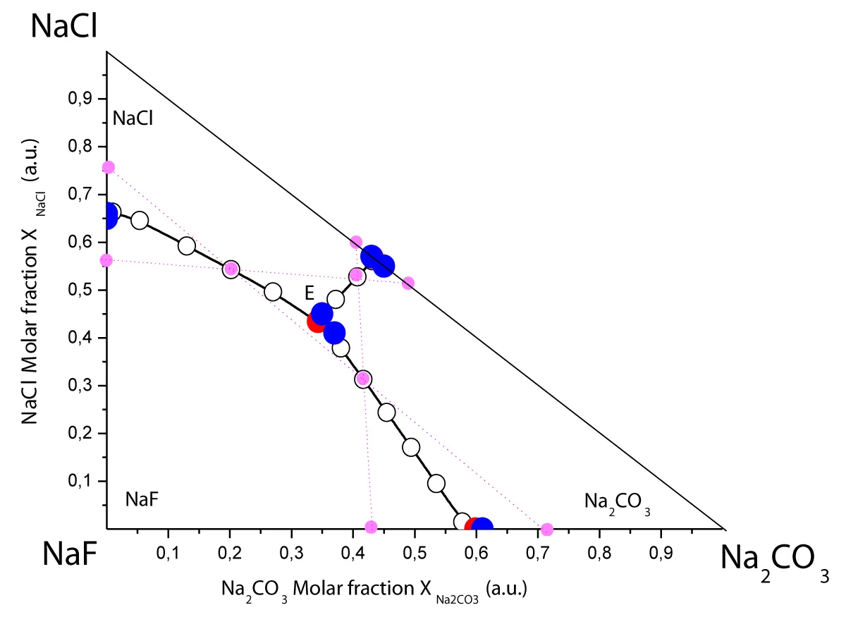
Figure 1: Fusibility diagram in ternary systems Na2C03 – NaF - NaCl (lines and hollow circles are geometrical calculations, red circles are calculated eutectics, blue circles are experimental data [28, 46, 47]). Purple dotted lines and circles demonstrate an algorithm for constructing mono-variant curves by intersecting straight isotherms of the liquidus (in the example in Figure 1, corresponding to a temperature of 910 K), E – ternary eutectic.
Earlier in [8], a non-model thermodynamic algorithm was developed for calculating thermodynamic functions (chemical potentials, activities, and partial pressures of volatile components – µi, ai, Pi) for given values of state parameters (temperature, total pressure, and chemical potential of solvent -water – T, P, µW) and constructing diagrams of liquid-water equilibria.pairs of quasi-simple systems, exclusively from data on binary subsystems i -W - aw (mi) The equations for calculating the activity of the i-th volatile component of the ternary solution - and have the following form:
(10)
(11)
Where at the given water activity (aw = const); – activity of i–th component in binary system i–W; – activity of i–th component in ternary system, Zi is the Yeneke index of the i–th component of the solution or the mole fraction in the solvate–free concentration space (see equation (8)), Pi – partial pressure of i–th volatile component in ternary system , – Henry constant of i–th volatile component, determined in binary subsystem i-W. Solvent partial pressure Pw, determined by Raul’s law [14]:
(12)
where: - the vapor pressure above the pure solvent under the conditions under consideration (tabulated, for example, for Н2О at 25°C, at P 1 atm. = 23.76 mm Hg). Sum vapor pressure, Psum, according to Dalton law:
(13)
Where, the summation is carried out for all volatile components and volatile solvent. An example of calculating the solubility diagram of the KCl – HCl – H2O system at 25°C is shown in Figure 2 in Supplement to the article. There are also quite rare direct experimental data on the partial pressures of volatile components from [15], which are in perfect agreement with the results of non-model calculations for binary systems. Algorithms for calculating solubility diagrams of systems with one, two, and three volatile components in ternary and quaternary quasi-simple systems are also demonstrated in [8].
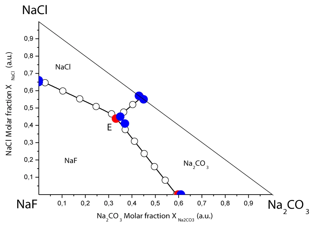
Figure 2: Fusibility diagram of the Na2C03 – NaF - NaCl ternary system (lines and hollow circles are thermodynamic calculations, red circles are calculated eutectic, blue circles are experimental data [28, 46, 47]), E is ternary eutectic.
The main goal of this article is to transfer the previously developed algorithm for calculating phase diagrams of multicomponent quasi-simple systems exclusively from data on binary subsystems of their components.
2. Thermodynamic substantiation of the algorithm for calculating the melting diagrams of quasi-simple systems
2.1. Consequence of fundamental thermodynamic equations
Intuitively, it is quite clear that in the case of quasi-simple ternary or more component systems, the thermodynamic properties must inevitably be completely determined by the properties of the binary subsystems that make up them. This fact follows directly from the need to fulfill the fundamental Gibbs–Duhem equation and the cross-differentiation conditions for the liquid phase of an n-component system under isothermal-isobaric conditions [9,10,16]:
(14)
(15)
Where: ni – the number of moles of the i-th component of the liquid phase of variable composition. In the case where the composition of the system belongs to the isopotential of a component (a solvent for solubility diagrams or one of the eqivalent components of the melt for fusibility diagrams, we assign the number n to this component), the equation is added to the system of differential equations (14), (15):
(16)
And in the case of quasi-simple systems, an equation belonging to a linear form of type (6) is added to these equations:
or (17)
Thus, excess thermodynamic functions in multicomponent liquid phases (component activities - ai, their chemical potentials - i), as well as diagrams of liquid-vapor phase equilibria (l-v), solubility and fusibility (s-l) diagrams of multicomponent systems should be calculated directly from data on thermodynamic functions of binary subsystems. Indeed, for example, for a three-component liquid phase n = 3, to describe the thermodynamic properties of the latter at T, P = const, it is sufficient to determine the functional dependence of the Gibbs potential G (n1, n2, n3)
To do this, it is enough to determine the values of 9 partial derivatives - , of which, only 3 are independent under the conditions under consideration (3 are excluded by conditions (15), and 3 more by belonging to a linear form L (17): ). The remaining 3 equations to determine - these are equations (14), (16) and an additional equation limiting the number of moles of the system components: when using the molar fraction scale in melts, or : when using the molality scale in solutions. Belonging to a specific liquidus temperature in the melting diagram or a specific solvent iso-potential line in the solubility diagram is determined by the value of the free term in linear form L - α0 (6) or the integration constant in differential form (17).
2.2. Topological isomorphism of phase diagrams and related works
The fact of the complete iso-structure of the Van-der-Waals differential equations is well known, describing diagrams of liquid-vapor phase equilibria (at constant temperature or pressure), fusibility diagrams (at constant pressure) and solubility diagrams (at constant temperature and pressure simultaneously) [4,17,18]. At the same time, the number of components in the solubility diagrams is 1 more, than in other diagrams to describe the solubility diagrams. To describe solubility diagrams, the metric of the Korzhinsky potential (or incomplete Gibbs potential, abbreviated for solvent) is used, which is characteristic in variables such as temperature, pressure, the number of moles of dissolved components, and the chemical potential of the solvent [4,19,20].
Other phase diagrams are described in the metric of the usual Gibbs potential, which is characteristic in variables such as temperature, pressure, and the number of moles of all system components. The consequence of the iso-structure of differential equations is a complete topological isomorphism of phase diagrams of various types, in particular, diagrams of solubility of (n+1)-component systems in variables: and fusibility diagrams in the variables: (where: – the vector of the solution composition in the reduced solvent-free concentration space of the Yenecke indixes, - the vector of the melt composition in the total concentration space of molar fractions). Thus, if the authors of [7,8] succeeded in developing a universal algorithm for calculating solubility diagrams and diagrams of liquid-vapor phase equilibria of quasi-simple systems, then the authors of this work have the right to assume that an analog of this algorithm exists for melting diagrams of quasi-simple systems.
2.3. Algorithms and methodology of model calculations
Another reason for searching for a thermodynamic method and algorithm for calculating the melting diagrams of quasi-simple systems is the fact that there are a number of model algorithms for calculating the phase diagrams of such systems. Here are just 2 examples.
V. Filippov and co-authors proposed a method for calculating solubility diagrams of ternary systems using K. Pitzer's equations [21,22] from data on binary subsystems [23,24]. Binary Pitzer parameters [21] are used to determine the compositions of binary solutions corresponding to different values of solvent activity . Then an artificial array is constructed from calculated rectilinear solvent isoactivates in a ternary system and the ternary parameters of the Pitzer equations are found [23]. Then, using the binary and ternary Pitzer parameters and the values of the thermodynamic potentials of the solid phases (determined by solubility in binary subsystems), the authors performed a trivial calculation of the solubility diagram of the ternary system. At the same time, the straightness of the isoactivated solvent does not mean that the ternary Pitzer parameters are equal to zero [4,23,24].
A similar example of model calculation of fusibility diagrams of ternary quasi-simple systems using the semi-empirical EFLCP model [25-27] is also associated with the following set of operations: model description of fusibility diagrams of binary subsystems and finding binary parameters of EFLCP; finding compositions of binary systems (corresponding to certain liquidus temperatures); construction of an artificial array T(X1,X2) and finding ternary parameters EFLCP; construction of fusibility diagram of ternary system.
The authors again believe that if it is possible to calculate diagrams of phase equilibria of multicomponent systems, using thermodynamically consistent semi-empirical models, then there may be a non-model method of such calculation.
2.4. Geometric method for calculating diagrams of quasi-simple systems
This calculation method is quite understandable. For such a calculation, it is sufficient to carry out the most accurate description of the fusibility diagrams of the binary subsystems of the multicomponent system under consideration, and in the temperature range corresponding to metastable super-cooled melts. Such a description can be carried out in various ways: from accurate direct experimental data (which is relatively rare), within the framework of any consistent thermodynamic model, or even using a simple mathematical model capable of extrapolation, for example, B-Spline. The only and main difference from the approaches described above in the section “Algorithms of model calculations” is the fact that we use algorithms or models for describing ternary systems, i.e. the use of moles is strictly limited to binary subsystems. For an example of calculation, consider a ternary salt system with a common cation.
2.5. System Na2CO3(1) – NaF (2) – NaCl(3)
This system is interesting because both for itself and for all its binary subsystems there are reliable and well-consistent experimental data on fusibility diagrams [28-45], and the system itself is quasi-simple with a very high probability and accuracy. To describe the fusibility diagrams of all three binary subsystems, we used a simple iso-osmotic model. The crystallization branch of the i-th component of the i-j system is valid:
(18)
where: - molar enthalpy of fusion of i-th component, – temperature of fusion, ai, Xi – activity and molar fraction of i-th component in saturated melt, – osmotic coefficient in the system i-j, independent on temperature and composition, .
(19)
where: – temperature functions of the molar isobaric heat capacity of the i-th component in the melt and solid phase, respectively, – it’s average values at .
Data on the properties of individual components, unified osmotic coefficients, and coordinates of binary eutectic are presented in Tables 1, 2, and Figure 3 of the Supplement. It is clearly seen from Figure 3 that the simplest isosmotic model is quite sufficient for an accurate description of the melting diagrams of binary subsystems.
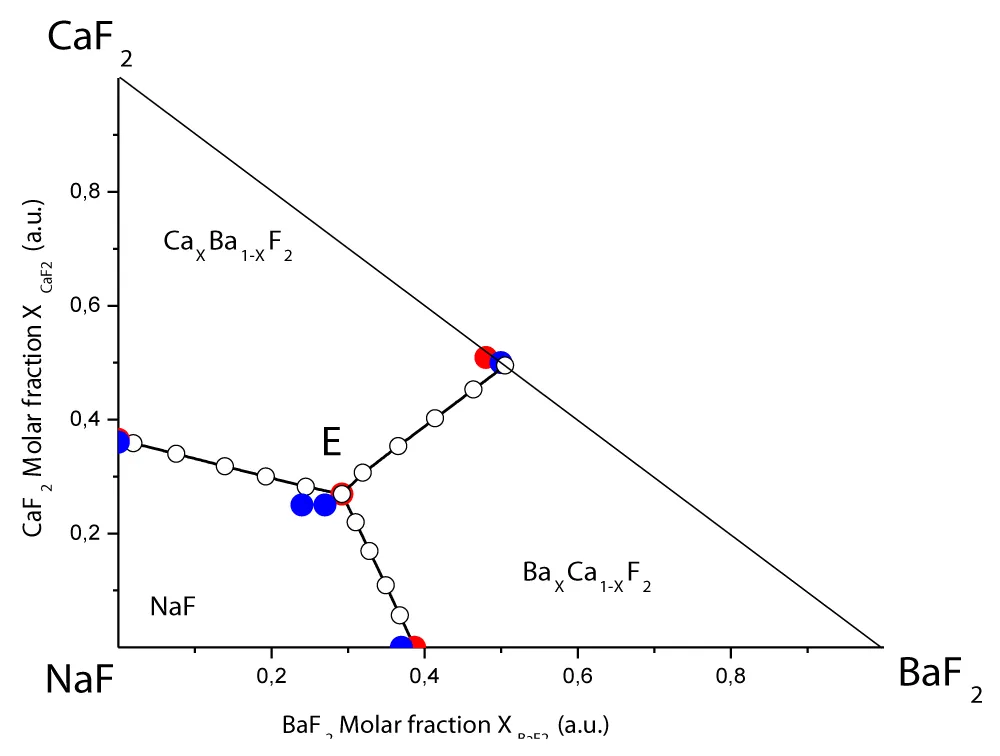
Figure 3: Fusibility diagram of the NaF - BaFZ2 – CaF2 ternary system (lines and hollow circles are thermodynamic calculations, red circles are calculated eutectic, blue circles are experimental data [28, 50-58]), E is the ternary eutectic.
Numerical calculated data on the melting diagrams of binary subsystems, including supercooled melts, are presented in Table 3 Applications. Let's take a closer look at the algorithm for calculating the melting diagram of a ternary system using the geometric method. Fix the temperature of the liquidus – T. The equations of the direct isotherms of the liquidus in the crystallization fields of different i-th solid phases (they are also iso-activates of the i-th components), written in segments, have the form:
NaCl – iso-activate: (20.1)
NaF –iso-activate: (20.2)
Na2CO3–iso-activate: (20.3)
where: X1, X2 – molar fractions of Na2CO3 and NaF in ternary melt;
– molar fraction of NaCl on the crystallization curve of NaCl in binary system NaCl - NaF ; – molar fraction of NaCl on the crystallization curve of NaCl in binary system NaCl - Na2CO3; – molar fraction of NaF on the crystallization curve of NaF in binary system NaF - NaCl; – molar fraction of NaF on the crystallization curve of NaF in binary system NaF - Na2CO3; – molar fraction of Na2CO3 on the crystallization curve of Na2CO3 in binary system Na2CO3 - NaCl; – molar fraction of Na2CO3 on the crystallization curve of Na2CO3 in binary system Na2CO3 - NaF (Table 3).
To calculate the monovariant curves of the joint crystallization of two salts consisting of points representing the intersections of two of the three liquidus isotherms, it is necessary to solve systems of 2 of 3 different equations of the lines (20.1) – (20.3). As a result, we obtain:
The branch of joint crystallization of NaCl+NaF – equations (20.1) and (20.2):
(21.1)
The branch of joint crystallization of NaF+Na2CO3 – equations (20.2) and (20.3):
(21.2)
The branch of joint crystallization of NaCl+Na2CO3 – equations (20.2) and (20.3):
(21.3)
The main calculation equations for geometrical method - equations (21.1) - (21.3) are related in trios. And all trios are independent. Each trio is responsible for calculating one monovariant curve (there are three in total), which must all intersect at one non-variant point. The results of calculating the melting diagram of the ternary system are presented in the Table 4 of Supplement and in article in Figure 1. The few experimental data available in the literature are also presented there for comparison. As can be seen from Figure 1 there is generally a fairly convincing agreement between the results of the geometric calculation and the experiment, which fully corresponds to the accuracy of the calculation in binary subsystems - Figure 3 in Supplement.
2.6. Substantiation of the basic formula of non-model calculation
The basic calculation formula is now justified by adapting the thermodynamic description of quasi-simple systems given in [7,8] to quasi-simple fusibility diagrams. So, let's consider an n-component melt of composition ( ) formed by mixing n binary melts of composition ( ) taken at the same temperature T, and during this mixing the temperature of the ternary solution did not change. It was shown earlier in [7,8] that the change in the Gibbs potential during the formation of such a quasi-simple multicomponent melt (Gmix) is determined only by the entropy of ideal mixing of binary melts at a given temperature (considered as quasi-components of a multicomponent system):
(22)
where: – activity of i-th component in a multicomponent and binary melt (1-i) of the same temperature, respectively, Zi is an analog of the Yenecke index in the solubility diagrams [7,8] and we retain the designation:
(23)
From (23) it follows, that:
(24)
which we will call the equation of quasi-simple systems. Let us now consider a ternary system (index ((ter = i-j-k)), namely, a branch of the joint crystallization of components (i-j) starting from a binary non-invariant eutectic point with coordinates: (Let us now apply the basic equation (24) to a ternary melt of composition at temperature T and a eutectic binary melt of composition :
(25)
Applying the reasoning to both components, we get:
(26)
Using equation (18): , we immediately obtain a system of equations for calculating the mono-variant crystallization branch of the components (i-j):
(27)
1. The system of equations (27) has a number of obvious advantages over the geometric method, in particular:It does not require any model description of binary subsystems;
2. More importantly, it does not require extrapolation of the crystallization branches of the components to sub-eutectic temperatures;
3. Allows you to directly (with a certain accuracy – see below) calculate all the coordinates of the trernary eutectic (corresponding to crystallization i-j-k components):
4. As strange as it may seem at once, system (27) allows us to check with what accuracy the system is quasi-simple, i.e. how rectilinear are the isotherms-isobars-isopotentials in it?
2.7. Thermodynamic method for calculating diagrams of quasi-simple systems. Results and discussion
The difference between the geometric method for calculating of fusibility diagrams (calculating the intersections of straight lines of liquidus isotherms) and the thermodynamic method for the same calculation is the absence of such a calculation and the need to extrapolate liquidus isotherms to supercooled metastable melts (here, only data on the coordinates of binary eutectics of subsystems are used).
To construct a melting diagram of the ternary i-j-k system, it suffices to solve 3 pairs of systems of equations of type (27) for 3 branches of joint crystallization of pairs of components:
(i-j):
(28.1)
(28.2)
(i-k):
(28.3)
(28.4)
(j-k):
(28.5)
(28.6)
A variant of the thermodynamic calculation of the melting diagram of the previously considered Na2CO3 - NaF - NaCl system is shown below in Figure 2 and in the Table 5 of Supplement.
As can be seen from Figures 1, 2 and Tables 4, 5, the thermodynamic calculation data as a whole are in convincing agreement with both the available experimental data and the result of the thermodynamic calculation, which, in general, is not surprising. However, the thermodynamic method, firstly, is an order of magnitude less laborious and does not require a large number of experimental data on the melting diagrams of binary subsystems for more or less accurate extrapolation (it requires only the coordinates of binary eutectic). To find the exact coordinates of the ternary eutectic
With 3 independent variables, it is necessary and sufficient to solve a system of three transcendental equations from the system (28.1)-(28.6) with respect to and 2 of the three eutectics molar fractions. There are 9 different solutions by the numbers of the selected equations (28.M)-(28.N)-(28.P): (M-N-P) = (1-2-3), (1-2-5), (2-3-5), (1-3-4), (1-3-6), (3-4-6), (2,4-6), (2-5-6), (4-5-6). Numerous calculations show, that, if the isotherms of the liquidus are really rectilinear and the coordinates of the binary eutectic are established accurately enough ; ; (then the coordinates of the ternary eutectic (the solution of 9 different variants of 3 of equations) are set with the same accuracy – see Table 5.
2.8. Restrictions on the use of the thermodynamic method
The only rather strict condition for the applicability of the thermodynamic calculation method is the requirement of “quasi-simplicity", i.e., the straightness of the liquidus isotherms. Very conditionally, we divide the considered ternary systems into formal classes:
2.8.1. If we consider ternary systems consisting of nonelectrolytes, for example, the fusibility diagrams of ternary oxide systems [48], the proportion of quasi-simple systems is, according to the authors, 3-5 rel. %.
2.8.2. If we consider ternary systems consisting of electrolytes, for example, the fusibility diagrams of ternary salt systems with a common cation or common anion [49], the share of such systems is estimated by the authors to be 5-7 rel. % for systems with a common cation and 2-4 rel. % for systems with a common anion.
2.8.3. In ternary inter-salt systems, the proportion of quasi-simple systems is quite small - 1-2 rel. % [49]. This is not surprising, since, unlike systems of classes 1 and 2, the liquidus isotherms in this case, in principle, cannot be absolutely linear even in simple eutectic systems. For example, at the Van Rijn points [4,12,17] (when the figurative points of the compositions of two solid phases and the melt in equilibrium with them are on the same straight line), the liquidus isotherms in the solid phase crystallization fields touch each other and the two-phase equilibrium is disrupted the curve. Thus, in at least 2 of the 4 solid phase crystallization regions, the liquidus isotherms cannot be absolutely linear. However, a number of ternary interaction systems still have a fairly simple set of liquidus isotherms in several crystallization regions at once.
2.8.4. If a mono-variant curve, involving a compound, is calculated, using a thermodynamic algorithm, then the absolute straightness of the liquidus isotherms in the crystallization fields is also incredible. Indeed, the latter should bend around the figurative junction point, forming closed curves (in the case of ternary junctions) or semi-closed curves cut off by the side of the concentration triangle (in the case of binary junctions).
2.8.5. If a number of solid solutions are formed in the system, the straightness of the liquidus isotherms is found in principle (although very infrequently ~ 2 rel.% [48,49]). However, in a system with a continuous series of solid solutions with points of extreme liquidus temperatures, straightness is also incredible, since the liquidus isotherms in this case either touch or bend around such figurative points.
2.8.6. Systems involving binary solid solutions with a wide miscibility gap may well be quasi-simple with rectilinear liquidus isotherms, similar to simple eutectic systems [48,49].
2.9. System NaF – BaFZ2 – CaF2
To demonstrate the possibilities of the thermodynamic calculation method using the example of the more rarely encountered fusibility diagram of a quasi-simple ternary system with a common anion in Figure 3, we present the calculation results in the NaF – BaFZ2 – CaF2 system. The data on the properties of the individual components of the system are presented in the Table 1 in Supplement, data on the compositions of binary eutectic substances are presented in the Table 6 in Supplement and also in Figure 3. Figure 3 also presents a few experimental data on the ternary system [28,58]. It is clearly seen that the thermodynamic calculation data are generally in convincing agreement with the available experimental data, despite the fact that one of the binary subsystems BaFZ2 – CaF2 implements a number of eutectic cubic solid solutions [56,57] with a wide range of immiscibility: CaXBa1-XF2. We estimated the regular non-ideality parameter within the framework of the LDM model [25]:
| Table 1: Calculated NaCl-NaF joint crystallization curve and ternary eutectics for 9 quasi-simple NaCl-NaF-X ternary systems. | |||||
| T(K) | XNaF (mol.fr.) |
XNaCl (mol.fr.) |
Xi (mol.fr.) |
Solid phases | References |
| 957 | 0,337 | 0.663 | 0.000 | NaF + NaCl | from [30], P.742, 743 |
| 805 | 0.120 | 0.330 | 0.550 | NaF + NaCl + Nal | [62]. From [49]. P.126. |
| 893 | 0.305 | 0.505 | 0.190 | NaF + NaCl + Na2S04 | [63]. From [49]. P.126-127. |
| 905 | 0.212 | 0.375 | 0.375 | NaF + NaCl + NaF + Na2S04 | [63]. From [49]. P.126-127. |
| 848 | 0.210 | 0.420 | 0.370 | NaF + NaCl + Na2C03 | [47]. From [49]. P.125. |
| 799 | 0.193 | 0.320 | 0.487 | NaF + NaCl + Na2C0r4 | [64]. From [49]. P. 126 |
| 561 | 0.050 | 0.080 | 0.8670 | NaF + NaCl + NaN03 | [65] |
| 937 | 0.330 | 0.639 | 0.031 | NaF + NaCl + SrF2 from Na, Sr//Cl, Br | [66]. From [49]. P.476. |
| 941 | 0.321 | 0.654 | 0.0125 | NaF + NaCl + CaF2 from Na, Sr//Cl, Br | [67]. From [49]. P.247. |
| 645 | 0.075 | 0.150 | 0.775 | NaF + NaCl + KV03 | [68] |
| 957 | 0,33700 | 0,66300 | 0,00000 | NaF + NaCl + X | Thermodynamic calculation |
| 950 | 0,32672 | 0,64600 | 0,02729 | ||
| 930 | 0,29826 | 0,59849 | 0,10325 | ||
| 910 | 0,27120 | 0,55262 | 0,17618 | ||
| 890 | 0,24554 | 0,50844 | 0,24603 | ||
| 870 | 0,22129 | 0,46600 | 0,31271 | ||
| 850 | 0,19846 | 0,42536 | 0,37618 | ||
| 830 | 0,17706 | 0,38656 | 0,43638 | ||
| 810 | 0,15708 | 0,34964 | 0,49328 | ||
| 790 | 0,13851 | 0,31464 | 0,54685 | ||
| 770 | 0,12134 | 0,28160 | 0,59706 | ||
| 750 | 0,10555 | 0,25054 | 0,64390 | ||
| 730 | 0,09112 | 0,22149 | 0,68739 | ||
| 710 | 0,07801 | 0,19445 | 0,72754 | ||
| 690 | 0,06619 | 0,16943 | 0,76439 | ||
| 650 | 0,04622 | 0,12540 | 0,82838 | ||
| 600 | 0,02759 | 0,08136 | 0,89105 | ||
| 550 | 0,01499 | 0,04880 | 0,93621 | ||
| 500 | 0,00721 | 0,02642 | 0,96637 | ||
(29)
where: standard heats of formation of compounds forming a solid solution (Given in the Supplement), a(i), a(j) – crystal lattice periods (a(CaF2) = 0.5451 nm; a(BaFZ2) = 0.6200 nm [60-62]). So, we obtained: α(S)(CaF2 - BaFZ2) = 82.6 kj/mole. Corresponding miscibility gap at the temperature of binary eutectic is: and at the temperature of ternary eutectic even wide: This circumstance practically does not affect the accuracy of the calculation by the proposed thermodynamic method.
3. A unified branch of the joint crystallization of two components in various quasi-simple systems. Methodology of calculation - Results and discussion
If we consider in detail the system of equations describing the construction of a mono-variant branch of the joint crystallization of two components (i-j) in a quasi-simple ternary system - (28.1), (28.2), then we can come to a rather paradoxical, at first glance, conclusion: All branches of the joint crystallization of the components (i-j) are fragments of the same mono-variant curve starting from the figurative point of the binary eutectic. On the other hand, this is expected, since the properties of a ternary system should be completely determined by the properties of binary subsystems. We will demonstrate a similar calculation of the NaCl - NaF joint crystallization curve in a set of 9 systems (of which 8 are ternary – see Figure 4). As can be seen from Figure 4, the NaCl-NaF crystallization lines for all quasi-simple NaCl - NaF-X ternary systemsms are indeed projected onto a single mono-variant curve with fairly high accuracy. At the same time, the temperatures of the eutectic correspond quite well to the calculated liquidus temperatures (including for 3 mutual systems). All these ternary non-variant points are represented also in summary Table 1.
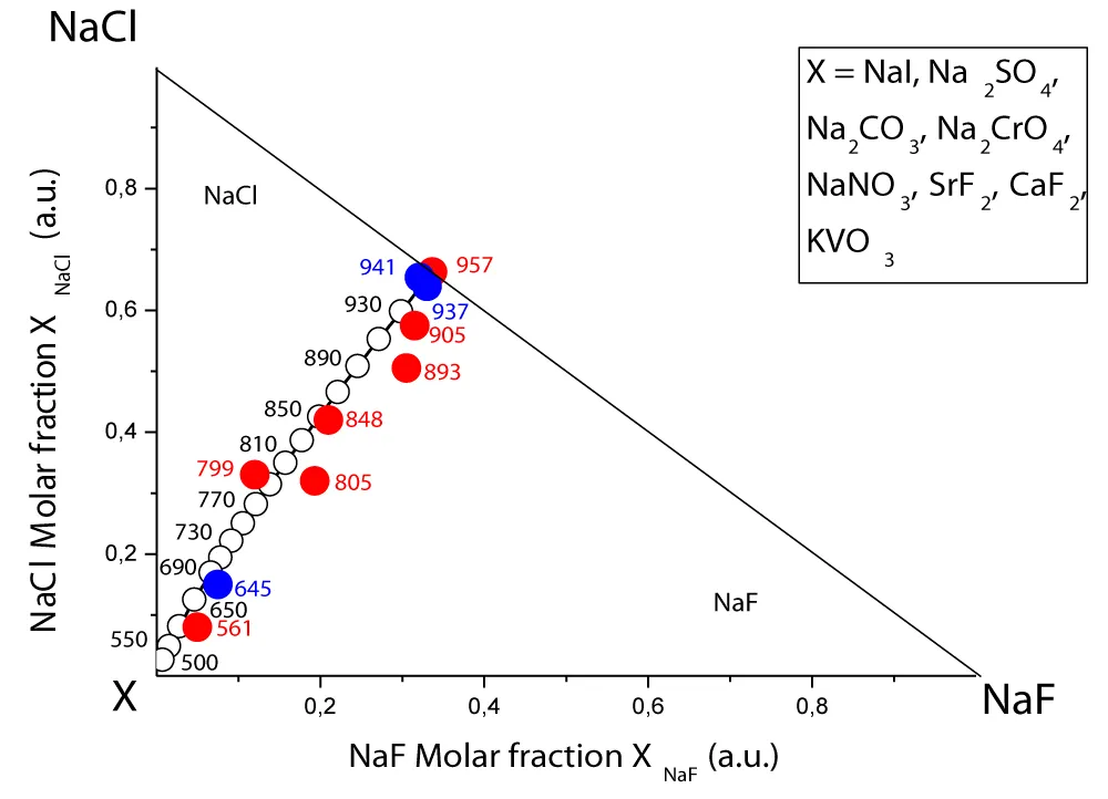
Figure 4: Calculated NaCl-NaF joint crystallization curve for 9 quasi-simple NaCl-NaF-X ternary systems (black lines and hollow circles are thermodynamic calculations, red circles are eutectic in ternary systems with a common cation, blue circles are eutectic in ternary reciprocal systems).
4. A method for verifying the compliance of ternary systems with the condition of quasi-simplicity - Straightness of liquidus isotherms
The a priori application of the thermodynamic calculation method is complicated by the obvious facts that:
4.1. There is clearly insufficient direct experimental data in the literature on the melting diagrams of ternary systems, although there is certainly a much larger set of such systems available to experiment compared to binary systems with the same components: (n – the number of available components of this class, for example, metal salts, oxides, sodium salts, fluorides ..., is usually in the tens, if not hundreds). Data on four or more component systems is even more relatively poor.
4.2. Often, even if data on monovariant and non-invariant equilibria are presented in the literature, data on liquidus isotherms in solid phase crystallization fields are absent or very scarce. There is practically no data on isothermal surfaces of the liquidus in four or more component systems.
4.3. Even if data on liquidus isotherms are available in ternary or more component systems, it is practically difficult to judge how reliable they are. For example, for data on fusibility diagrams at high temperatures (in which obtaining such data is the most laborious and least accurate), the liquidus isotherms are artificially straightened or constructed more or less arbitrarily based on data on binary subsystems.
4.4. In any case, it is often difficult, if not impossible, to reliably judge whether a multicomponent system is quasi-simple based on direct experimental data on binary subsystems. The question arises whether it is possible to judge how quasi-simple system is using only data on binary subsystems. Judging by the very formulation of the problem, such a method may exist. Indeed, we will use the basic system of equations (28.1)-(28.6) and calculate the pairwise differences of equations (28.1) and (28.3); (28.2) and (28.5); (28.4) and (28.6). As a result, we obtain the following system of equations:
(30.1)
(30.2)
(30.3)
where: – temperature of binary eutectic in subsystem (i - j); – molar fraction of i-th component in binary eutectic in subsystem (i - j); ∆Qi – modulus of deviation from the condition of quasi-simplicity (straightness of liquidus isotherms in a ternary system(i – j - K), calculated from the i-th component. If the ternary system is ideally quasi-simple, and the coordinates of all binary eutectics, as well as the functional dependences of the melting heats of all components, are absolutely accurate, then: ∆Qi = ∆Qj = ∆Qk = 0. Naturally, in reality this is unattainable. We will carry out the appropriate calculation for specific systems.
4.5.1. System Na2CO3 – NaF – NaCl: Let's evaluate the result. To do this, we will perform an estimated calculation. Let's take the conditional temperature of the eutectic , typical error in its definition , typical heat of fusion . Then, the expected error in the function definition is Corresponding error of the entire temperature part of the function ∆Qj: . The value of the concentration of the i-th component in a binary eutectic with its participation is generally uncertain: However, values close to 0.0 are nevertheless absolutely atypical, since eutectics belong to the very branch of crystallization of the i-th component. Let's take a fairly low value for certainty. (which gives the maximum error in the calculation): , and the expected error in its determination Then expected error in its determination The corresponding error of the entire concentration part of the function ∆Qi: . In total, the expected error in defining the entire function is δ∆Qi ~ 0.14. Thus, it can be stated that the system under consideration is really quasi-simple, and the coordinates of the binary eutectic are quite accurate. In the following, we assume the condition that the ternary system is quasi-simple - functions for all components: ∆Qi ≤ 0.20.
4.5.2. System NaF – BaFZ2 - CaF2: In this system with a common anion (which are less often and less accurately quasi-simple), the following values are obtained: Thus, this system also seems to the authors to be really quasi-simple, although with noticeably lower accuracy compared to the previous one. The latter may be related to the formation of binary solid solutions in the system: CaXBa1-XF2 with a very wide miscibility gap.
4.5.3. System LiF – NaF - RbF: In conclusion, let us consider another ternary fluoride system, which is not quasi-simple. For it, the calculation based on experimental data on binary eutectic [69-73] gives the following values: Thus, this system is in no way quasi-simple.
The quasi-simplicity criterion we present was obtained by examining several hundred systems of several classes (electrolyte and hydrocarbon non-electrolyte), and it is undoubtedly arbitrary. In the crystallization fields of compounds of constant composition, it cannot be applied in principle, since the liquidus isotherms in them are a priori nonlinear—they bend around the figurative junction point (at eutectic equilibria) or partially bend around it at peritectic equilibria. But even in such systems, quasi-simple parts of the systems can be encountered in the crystallization fields of individual components. If liquidus temperature extremes are realized in the diagrams of binary solid solutions, then the liquidus isotherms again cannot be linear, and the quasi-simplicity of such parts of the fusibility diagrams is impossible. This is because at such points, the liquidus isotherms touch the sides of the concentration triangle and cannot be linear.
In conclusion, as an example, we present a similar calculation of the melting diagrams of quasi-simple ternary systems, based on hydrocarbons - alkanes (C5-C10) (Figure 5-9). As can be seen from Figures 5-9, these experimental data [74-76] are in quite convincing agreement with the calculations using the non-model algorithm for quasi-simple systems proposed by the authors. Data on the heats of fusion of hydrocarbons are taken from [81-93] and are presented in Table S7 of the Supplement.
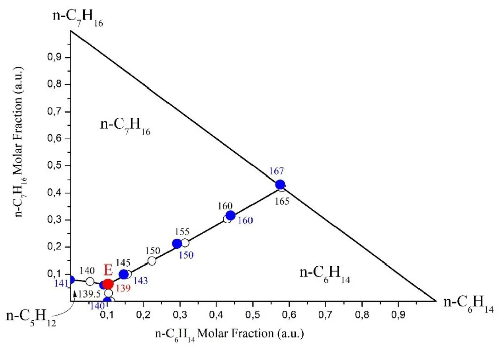
Figure 5: Fusibility diagram in ternary system n-C5H12 - n-C6H14 - n-C7H16: black lines and open circles – calculation; red point – eutectic nonvariant point (terminology – see [77-80]); blue circles - experimental data [74-76]; liquidus temperatures (K) are represented by figures.
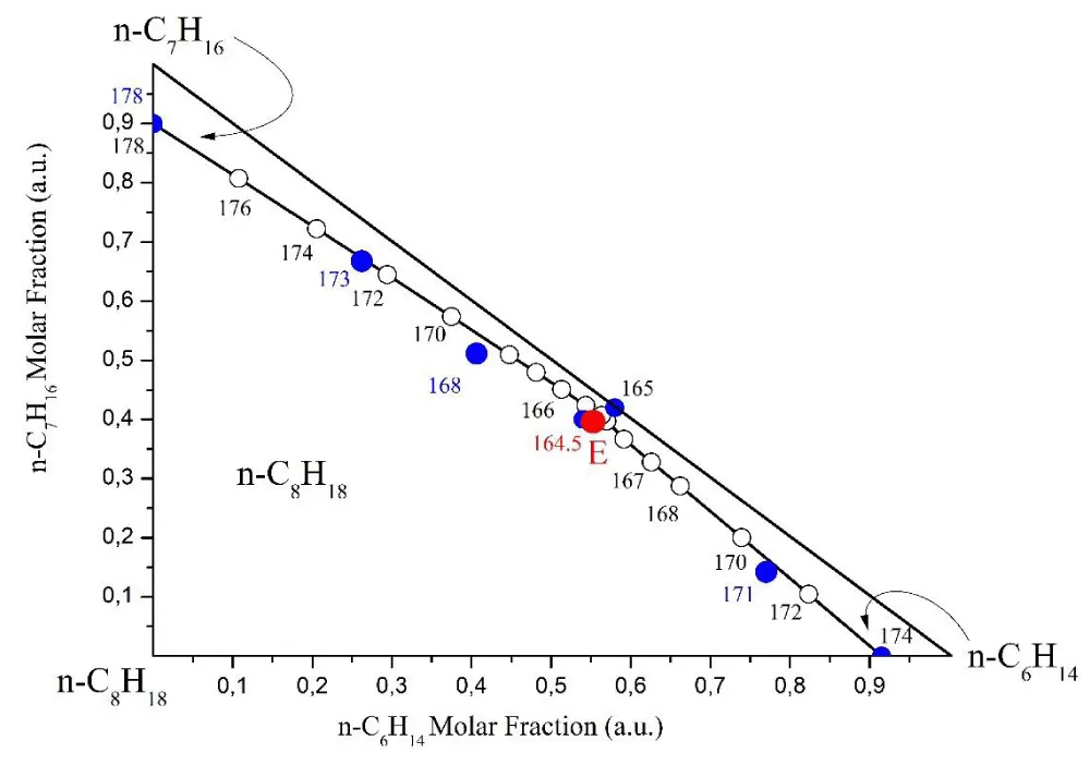
Figure 6: Fusibility diagram in ternary system n-C8H18 - n-C6H14 - n-C7H16: black lines and open circles – calculation; red point – eutectic nonvariant point (terminology – see [77-80]); blue circles - experimental data [74-76]; liquidus temperatures (K) are represented by figures.
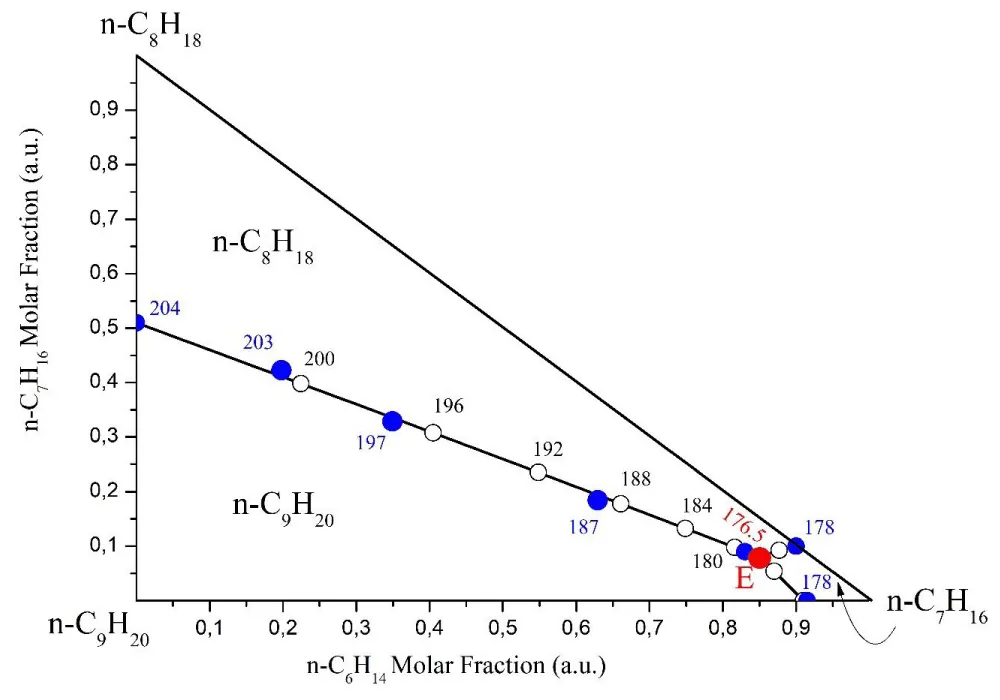
Figure 7: Fusibility diagram in ternary system n-C9H20 - n-C8H18 - n-C7H16: black lines and open circles – calculation; red point – eutectic nonvariant point (terminology – see [77-80]); blue circles - experimental data [74-76]; liquidus temperatures (K) are represented by figures.
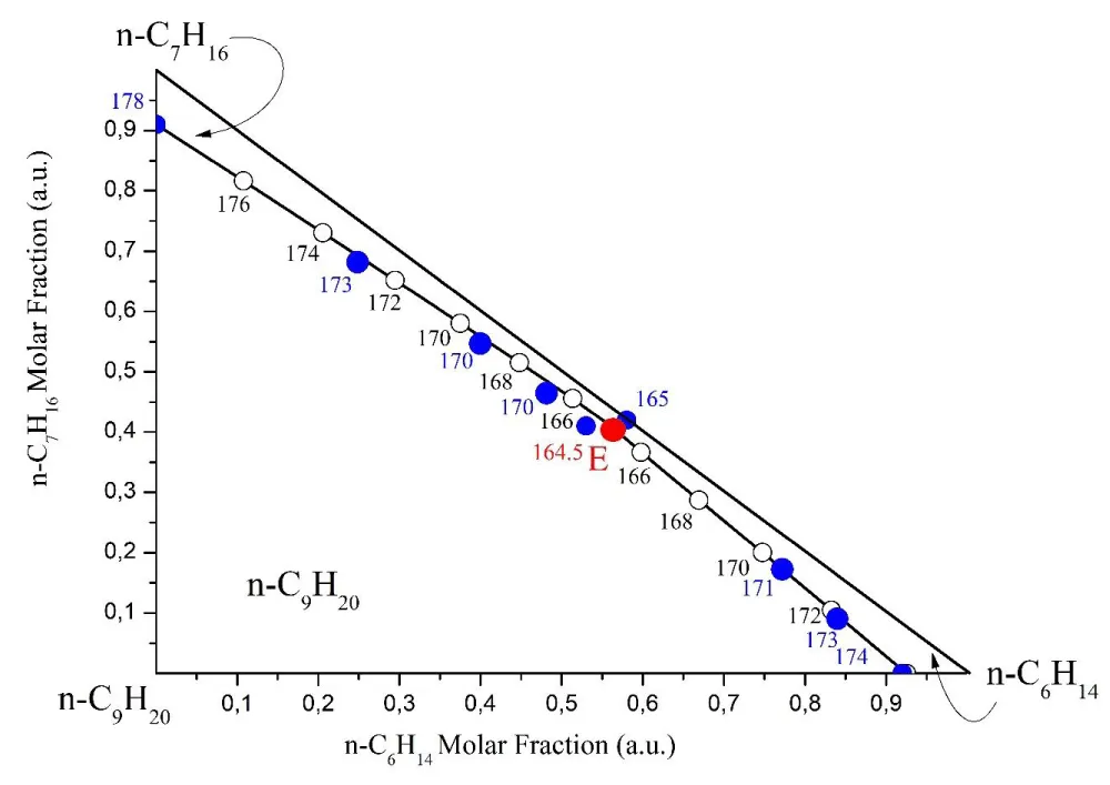
Figure 8: Fusibility diagram in ternary system n-C9H20 - n-C6H14 - n-C7H16: black lines and open circles – calculation; red point – eutectic nonvariant point (terminology – see [77-80]); blue circles - experimental data [74-76]; liquidus temperatures (K) are represented by figures.
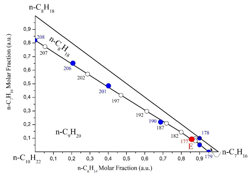
Figure 9: Fusibility diagram in ternary system n-C10H22 - n-C8H18 - n-C7H16: black lines and open circles – calculation; red point – eutectic nonvariant point (terminology – see [77-80]); blue circles - experimental data [74-76]; liquidus temperatures (K) are represented by figures.
The paper presents a non-model algorithm for calculating the fusibility diagrams of multicomponent quasi-simple systems (with linear liquidus isotherms in the crystallization fields of components) exclusively from data on the fusibility diagrams of binary subsystems, which make up these systems. The application of the algorithm is demonstrated by the example of fusibility diagrams of ternary quasi-simple salt systems with a common cation and a common anion. On the other hand, there is a convincing agreement between the calculation results and the available experimental data in the literature. The proof of the fact that all non-variant points of various quasi-simple ternary systems (with two identical and one different component) belong to one mono-variant curve is given. A system of transcendental equations has been compiled for calculating the coordinates of ternary eutectic systems from data on binary eutectic systems of quasi-simple subsystems. A thermodynamic method for determining whether a multicomponent system belongs to the class of quasi-simple systems is proposed.
Authors acknowledge that the primary focus on calculating complex phase diagrams of multicomponent systems currently relies almost exclusively on model-based (usually semi-empirical) calculation methods, and recently even on artificial intelligence. Articles in the highly respected journal CALPHAD brilliantly confirm this. After reviewing issues from the past five years, we simply couldn't find even a statement about calculating phase diagrams based on first principles of thermodynamics: the principles of thermodynamics, conditions of phase and chemical equilibrium, stability criteria, etc. Our method, however, exclusively utilizes such non-model assumptions and therefore seems to the authors worthy of at least some attention.
Financial support
Investigations are supported by Grant PCF BR24992786 “Development of Technology for Manufacturing Domestic Medical Instruments and Medical Devices”
Conflict of interests: Authors declare the absence of a conflict of interest.
Contribution of the authors
N.A.C., V.A.K, M.V.K. - conceptualization, development of thermodynamic algorithm; N.A.K., M.S., D.V.K. – development of geometrical algorithm of calculation; B.N.A., D.S.D, - selection and verification of experimental data; M.V.C, M.C.K, M.Yu.A, K.R – thermodynamic calculations.
- Zdanovskiy AB. Patterns in changing the properties of mixed solutions. Proceedings of the Salt Laboratory, Academy of Sciences of the USSR. 1936;(6):70 p.
- Ryazanov MA. Selected Chapters of the Theory of Solutions. Syktyvkar: Syktyvkar State University; 1997. 205 p.
- Mikulin GI. Thermodynamics of Mixed Solutions of Strong Electrolytes. Leningrad: Chemistry; 1968. p. 202–231.
- Charykova MV, Charykov NA. Thermodynamic Modeling of Evaporative Sedimentation Processes. St Petersburg: Nauka; 2003. 261 p. Available from: https://www.researchgate.net/publication/335623004_Thermodynamic_modeling_of_evaporation_processes_of_lunar_and_meteorite_substance
- Filippov VK. Systems obeying Zdanovskiy’s rule. Bulletin of Leningrad State University. Physics and Chemistry Series. 1977;(3):98–105.
- Wang Zh. The linear concentration rules at constant partial molar quantity Ψ₀ – extension of the Turkdogan and Zdanovskii rules. Acta Metallurgica Sinica. 1980;16(2):195–206. (In Chinese). Available from: https://www.ams.org.cn/EN/Y1980/V16/I2/195
- Charykov NA, Rumyantsev AV, Keskinov VA, Letenko DG, Charykova MV, Keskinova MV. Algorithm (procedure variants) for calculation of solubility diagrams of quasi-simple multicomponent water-electrolyte systems. J Chem Eng Data. 2024;69:4089–4097.Available from: https://doi.org/10.1021/acs.jced.4c00307
- Charykov NA, Rumyantsev AV, Keskinov VA, et al. A universal algorithm for calculation of vapor–liquid equilibrium diagrams in quasi-simple multicomponent systems. Condensed Matter and Interphases. 2025;27(1):67–85. Available from: https://doi.org/10.17308/kcmf.2025.27/12491
- Storonkin AV, Potemin SS. Issues of thermodynamics of eutectic and peritectic systems. In: Issues of Thermodynamics of Heterogeneous Systems and Theory of Surface Phenomena. Issue 4. Leningrad: Leningrad State University; 1977. p. 85–137.
- Storonkin AV, Potemin SS. Thermodynamic conditions of pseudo-ideality of ternary heterogeneous systems. In: Issues of Thermodynamics of Heterogeneous Systems and Theory of Surface Phenomena. Issue 7. Leningrad: Leningrad State University; 1985. p. 53–70.
- Storonkin AV. Thermodynamics of Heterogeneous Systems. Book 1: Parts I–II. Leningrad: Leningrad State University; 1967. 467 p. Available from: https://www.researchgate.net/publication/226120379_Thermodynamics_of_heterogeneous_systems_with_chemical_interaction
- Stonorin AV. Thermodynamics of Heterogeneous Systems. Book 2: Part III. Leningrad: Leningrad State University; 1969. 270 p. Available from: https://www.researchgate.net/publication/226120379_Thermodynamics_of_heterogeneous_systems_with_chemical_interaction
- Kogan VB, Ogorodnikov SK, Kafarov VV. Handbook of Solubility. Vol. 3: Ternary and Multicomponent Systems Formed by Inorganic Substances. Book 2. Leningrad: Nauka; 1969. 1171 p.
- Prausnitz JM, Lichtenthaler RN, De Azevedo EG. Molecular Thermodynamics of Fluid-Phase Equilibria. 3rd ed. New Jersey: Prentice Hall PTR; 1999. 860 p. Available from: https://www.psgraw.com/wp-content/uploads/2022/05/Molecular-Thermodynamics-of-Fluid-Phase-equilibria-3Ed.pdf
- Storonkin AV, Markuzin NP. Investigation of vapor pressure of saturated and unsaturated solutions of potassium chloride in hydrochloric acid. Zhurnal Fizicheskoy Khimii. 1955;29(1):111–119. (In Russian).
- Münster A. Chemical Thermodynamics. Moscow: Nauka; 1971. 340 p.
- Charykov NA, Rumyantsev AV, Semenov KN, et al. Topological isomorphism of liquid–vapor, fusibility, and solubility diagrams: analogues of Gibbs–Konovalov and Gibbs–Rooseboom laws for solubility diagrams. Processes. 2023;11(5):1405. Available from: https://doi.org/10.3390/pr11051405
- Charykov NA, Semenov KN, Keskinov VA. Non-variant phenomena in heterogeneous systems: new type of solubility diagrams points. Ann Adv Chem. 2023;7(1):74–97. Available from: https://doi.org/10.3390/pr1105140510.29328/journal.aac.1001047
- Filippov VK, Sokolov VA. Thermodynamics of Heterogeneous Systems and Theory of Surface Phenomena. Vol. 8. Leningrad: Leningrad State University; 1988. p. 39. (In Russian)
- Korjinskiy AD. Theoretical Basis of the Analysis of Mineral Paragenesis. Moscow: Nauka; 1973. (In Russia)
- Pitzer KS. Thermodynamics of electrolytes. I. Theore tical basis and general equations. J Phys Chem. 1973;77(2):268–277. Available from: https://doi.org/10.1021/j100621a026
- Pitzer KS, Kim JJ. Thermodynamics of electrolytes IV. Activity and osmotic coefficients for mixed electrolytes. J Am Chem Soc. 1974;96(18):5701–5707. Available from: https://doi.org/10.1021/ja00825a004
- Filippov VK, Charykov NA. Phase equilibria in the Na,Co // Cl,SO₄–H₂O system at 25°C. Russ J Appl Chem. 1986;59(11):2448–2453. Available from: https://www.researchgate.net/publication/293078200_Phase_equilibria_in_the_NaKMgCaSO4Cl-H2O_system_at_25C_in_the_phase_field_of_polyhalite
- Filippov VK, Charykov NA. Phase equilibria in the Na,Ni // Cl,SO₄–H₂O system at 25°C. Russ J Inorg Chem. 1988;33(5):1326–1330. Available from: https://www.researchgate.net/publication/357360376_Phase_Equilibria_in_the_Quinary_Na_MgCl_SO4_NO3-H2O_System_at_25C
- Mikhailova MP, Litvak AM, Charykov NA, Yakovlev YP. [Title unclear]. Russ Phys Tech Semiconductors. 1997;31(4):410–415. Available from: https://www.researchgate.net/publication/332578578_Discovery_of_III-V_Semiconductors_Physical_Properties_and_Application
- Litvak AM, Charykov NA. A new thermodynamic method for calculating melt–solid phase equilibria (ASWU systems). Zhurnal Fizicheskoy Khimii. 1990;64(9):2331–2335.
- Litvak AM, Charykov NA. A new thermodynamic method for calculating phase diagrams of binary and ternary systems containing In, Ga, As, and Sb atoms. Reports of the Academy of Sciences of the USSR. Inorganic Materials Series. 1991;27(2):225–230.
- Storonkin AV, Vasilkova IV. Questions of the thermodynamics of ternary eutectic and peritectic systems. Issues of Thermodynamics of Heterogeneous Systems and Theory of Surface Phenomena. 1971;(1):3–51.
- Grjotheim K, Halvorsen T, Holm JL. The phase diagram of the system NaF–NaCl and thermodynamic properties of fused mixtures. Acta Chem Scand. 1967;21(8):2300–2301. Available from: https://scispace.com/pdf/the-phase-diagram-of-the-system-naf-nacl-and-thermodynamic-3awnaogcdz.pdf
- Voskresenskaya NK, Evseeva NN, Berul SI, Vereschagina IP. Handbook on the Fusibility of Salt Systems. Vol. 1: Binary Systems. Moscow–Leningrad: Academy of Sciences of the USSR; 1961.
- Plato W. Z. Phys Chem. 1907;58:350. Cited in ref. 30:742.
- Wolters A. Neues Jahrb Mineral Geol Palaeontol Beil Bd. 1910;30:55. Cited in ref. 30:742.
- Bukhalova GA. Report of Sector of Physico-Chemical Analysis. 1955;26:138. Cited in ref. 30:743.
- Rassonskaya IS, Bergman AG. Reports of the Academy of Sciences of the USSR. 1943;38:238. Cited in ref. 30:743.
- Rea RF. J Am Ceram Soc. 1938;21:98. Cited in ref. 30:743.
- Le Chatelier H. C R Acad Sci. 1894;118:709. Cited in ref. 30:734.
- Sackur O. Z Elektrochem Angew Phys Chem. 1910;16:649. Cited in ref. 30:734.
- Sackur O. Z Phys Chem. 1912;78:550. Cited in ref. 30:735.
- Amadori M. Atti R Accad Lincei. 1913;22(5):366. Cited in ref. 30:735.
- Niggli P. Z Anorg Allg Chem. 1919;106:126. Cited in ref. 30:735.
- Jiang Y, Sun Y, Liu M, Bruno F, Li S. Eutectic Na₂CO₃–NaCl salt: A new phase change material for high-temperature thermal storage. Sol Energy Mater Sol Cells. 2016;152:155–160. Available from: https://doi.org/10.1016/j.solmat.2016.04.002
- Manoilov KE, Smirnov MN. Works of the All-Union Al–Mg Institute. 1940;22:98. Cited in ref. 30:738.
- Schmitz-Dumont O, Heckman I. Z Anorg Chem. 1949;260:49. Cited in ref. 30:738.
- Volkov NN, Shvab TF. Reports of Physico-Chemical Research Institute of Irkutsk State University. 1953;2(1):60. Cited in ref. 30:738.
- Volkov NN, Bergman AG. Reports of the Academy of Sciences of the USSR. 1942;35:50. Cited in ref. 30:738.
- Voskresenskaya NK, Evseeva NN, Berul SI, Vereschagina IP. Handbook on the Fusibility of Salt Systems. Vol. 1. Moscow–Leningrad: Academy of Sciences of the USSR; 1961. Available from: https://archive.org/stream/physicalproperti611janz/physicalproperti611janz_djvu.txt
- Volkov NM, Bergman AG. Reports of the Academy of Sciences of the USSR. 1940;27:967. Cited in ref. 46:125.
- Barzakovsky VP, Lapin VV, Boikova AI, Kurtseva NN. Diagrams of the State of Silicate Systems. Issue IV: Ternary Oxide Systems. Leningrad: Nauka; 1974. 514 p. Available from: https://apps.dtic.mil/sti/citations/AD0787517
- Voskresenskaya NK, Evseeva NN, Berul SI, Vereschagina IP. Handbook on the Fusibility of Salt Systems. Vol. 1. Moscow–Leningrad: Academy of Sciences of the USSR; 1961. Available from: https://archive.org/stream/physicalproperti611janz/physicalproperti611janz_djvu.txt
- Grjotheim K, Halvorsen T, Holm JL. Acta Chem Scand. 1967;21(8):2300–2301. Available from: https://actachemscand.ki.ku.dk/doi/10.3891/acta.chem.scand.21-2300
- Jiang Y, Sun Y, Liu M, Bruno F, Li S. Sol Energy Mater Sol Cells. 2016;152:155–160. Available from: https://doi.org/10.1016/j.solmat.2016.04.002
- Grube G. Z Elektrochem Angew Phys Chem. 1927;33:481. Cited in ref. 30:132.
- Bergman AG, Banashek EI. Reports of the Physical-Chemical Analysis Sector. 1953;22:196. Cited in ref. 30:133.
- Manoilov KE, Smirnov MN. Works of the All-Union Aluminum-Magnesium Institute. 1942;22:98. Cited in ref. 30:196.
- Rea RF. J Am Ceram Soc. 1938;21:98. Cited in ref. 30:196.
- Fuseya G, Mori M, Immura H. J Soc Chem Ind Jpn. 1933;36:175. Cited in ref. 30:128.
- Bukhalova GA, Bergman AG. Russ J Gen Chem. 1951;21:1570. Cited in ref. 30:128.
- Bukhalova GI. Russ J Inorg Chem. 1961;6:2359.
- Patnaik P. Handbook of Inorganic Chemicals. New York: McGraw-Hill; 2002. ISBN:0-07-049439-8.
- Gerward L, Olsen JS, Steenstrup S, Malinowski M, Osbrink S, Waskowska A. A high-pressure X-ray diffraction study of CaF₂. J Appl Crystallogr. 1992;25:578–581. Available from: https://doi.org/10.1107/S0021889892004096
- Hohnke DK, Kaiser SW. Epitaxial PbSe and Pb₁₋ₓSₓSe: growth and electrical properties. J Appl Phys. 1974;45(2):892–897. Available from: https://doi.org/10.1063/1.1663334
- Nagornyi HI. Report of the Sector of Physico-Chemical Analysis. 1938;11:291. Cited in ref. 49:126.
- Wolters H. Neues Jahrb Mineral Geol Palaeontol Beil Bd. 1910;30:50–127. Cited in ref. 49:126–127.
- Rassonskaya IS, Bergman AG. Rep Acad Sci USSR. 1943;48:238. Cited in ref. 49:126.
- Babev BD. System NaF–NaCl–NaNO₃. Inorg Mater. 2002;38(1):83–84. https://doi.org/10.1023/A:1013667914658
- Bukhalova GI. Sector of Physico-Chemical Analysis. 1955;26:268. Cited in ref. 49:476.
- Ichaque M. Bull Soc Chim Fr. 1952;(1–2):127. Cited in ref. 49:247.
- Gamataeva BY, Bermurzaeva ZI, Gamataev TSh, Gasanaliev AM, Salpagarova ZI. Phase equilibrium in NaF–NaCl–KVO₃ system. Dagestan State Pedagogical University Bulletin. 2015;(4):6–9.
- Bergman AG, Dergunov EP. Rep Acad Sci USSR. 1947;58:1369. Cited in ref. 30:475.
- Volkov NN, Tumash GP. News of the Physico-Chemical Institute at Irkutsk University. 1953;2(1):60. Cited in ref. 30:475.
- Dergunov EP. Rep Acad Sci USSR. 1941;31:752. Cited in ref. 30:475.
- Volkov NN, Shvab TF. News of the Physico-Chemical Institute at Irkutsk University. 1953;2(1):41. Cited in ref. 30:475.
- Dergunov EP. Rep Acad Sci USSR. 1947;58:1369. Cited in ref. 30:539.
- Zheleznyak AV. Physical-Chemical Properties of Hydrocarbon Systems with Carbon Numbers C5–C10. Abstract of PhD Dissertation. Krasnodar, Russia; 2006. 22 p.
- Zheleznyak AV. Physical-Chemical Properties of Hydrocarbon Systems with Carbon Numbers C5–C10. PhD Dissertation. Krasnodar, Russia; 2006. 220 p.
- Zheleznyak AV, Martsinkovsky AV, Danilin VN. Investigation of the fusibility diagram of the ternary pentane–hexane–heptane system. Physicochemical Analysis of Properties of Multicomponent Systems. 2006;(4):2.
- Azamatov BN, Charykov NA, Kuznetsov VV, Kulenova NA, Sadenova MA, Dogadin DS, Keskinov VA, Keskinova MV. Calculation of melting diagrams of a quasi-simple model of ternary systems: algorithm and thermodynamic justification. Phys Solid State. 2025;67(12):2464–2467. https://doi.org/10.21883/0000000000
- Charykov NA, Kulenova NA, Sadenova MA, Kuznetsov VV, Azamatov BN, Dogadkin DS, Charykova MV, Keskinova MV, Keskinov VA. Non-model calculation of fusion diagrams for quasi-simple systems from binary subsystem data. Russ J Inorg Chem. 2026;71(2):243–256. https://doi.org/10.1134/S0036023625601412
- Charykov NA, Kulenova NA, Sadenova MA, Azamatov BN, Dogadkin DS, Rumyantsev AV, Charykova MV, Keskinova MV, Keskinov VA. Unification of solubility diagrams of multicomponent quasi-simple systems. J Mol Liq. 2025;438:128614–128627. https://doi.org/10.1016/j.molliq.2025.128614
- Charykov NA, Kulenova NA, Sadenova MA, Kuznetsov VV, Azamatov BN, Dogadkin DS, Charykova MV. Unifying solubility diagrams of multicomponent quasi-simple systems. Russ J Phys Chem A. 2025;99(13):3302–3319. https://doi.org/10.1134/S0036024425702802
- Calculations, datasheets, CAD blocks, and other resources related to science and its subdisciplines. Available from: https://www.piping-designer.com/disciplines/chemical/chemical-elements/4060-pentane
- Pentane. NOAA CAMEO Chemicals. Available from: https://cameochemicals.noaa.gov/chris/PTA.pdf
- Hexane. Available from: https://www.piping-designer.com/disciplines/chemical/chemical-elements/4050-hexane
- n-Hexane. NOAA CAMEO Chemicals. Available from: https://cameochemicals.noaa.gov/chris/HXA.pdf
- Heptane. NOAA CAMEO Chemicals. Available from: https://cameochemicals.noaa.gov/chris/HPT.pdf
- Heptane (CID 8900). PubChem Compound Summary. Available from: PubChem Heptane ; Heptane. NIST Chemistry WebBook. Available from: https://webbook.nist.gov/cgi/cbook.cgi?ID=C111659&Mask=E
- Parks GS, Huffman HM, Thomas SB. Thermal data on organic compounds. VI. Heat capacities, entropies, and free energies of saturated non-benzenoid hydrocarbons. J Am Chem Soc. 1930;52:1032–1041.
- Domalski ES, Hearing ED. Heat capacities and entropies of organic compounds in the condensed phase. J Phys Chem Ref Data. 1996;25(1):1. Available from: https://doi.org/10.1063/1.555985
- Mondieig D, Rajabalee F, Metivaud V, Oonk HAJ, Cuevas-Diarte MA. n-Alkane binary molecular alloys. Chem Mater. 2004;16(5):786–798. Available from: https://doi.org/10.1021/cm031169p
- Nonane. NOAA CAMEO Chemicals. Available from: cameochemicals.noaa.gov›chris/NAN.pdf
- Nonane. Available from: https://www.stenutz.eu/chem/solv6.php?name=nonane
- Huffman HM, Parks GS, Barmore M. Thermal data on organic compounds. X. Further studies on heat capacities, entropies, and free energies of hydrocarbons. J Am Chem Soc. 1931;53:3876–3888.
- Decane. Available from: stenutz.eu›chem/solv6.php?name=decane