
More Information
Submitted: May 16, 2023 | Approved: June 19, 2023 | Published: June 20, 2023
How to cite this article: Cerdà V, Phansi P. Buffer Solutions of known Ionic Strength. Ann Adv Chem. 2023; 7: 051-056.
DOI: 10.29328/journal.aac.1001043
Copyright License: © 2023 Cerdà V, et al. This is an open access article distributed under the Creative Commons Attribution License, which permits unrestricted use, distribution, and reproduction in any medium, provided the original work is properly cited.
Keywords: pH calculation; Brömsted method; Buffer; Ionic strength

Buffer Solutions of known Ionic Strength
Víctor Cerdà1* and Piyawan Phansi2
1Sciware Systems, SL. Bunyola. 07193. Spain
2Department of Chemistry, Faculty of Science and Technology, Thepsatri Rajabhat University, Lopburi 15000, Thailand
*Address for Correspondence: Víctor Cerdà, Sciware Systems, SL. Bunyola. 07193. Spain, Email: [email protected]
pH buffer solutions are those in which minimal pH variations occur when moderate amounts of strong acids or bases are added or diluted. The most common buffers are those used in the intermediate pH zone and are made up of an acid-base conjugate pair (HA/A-), with Ca and Cb as analytical concentrations of acid and base respectively. The buffer capacity of a solution is the measure of its effectiveness in preserving the pH value when adding an acid or a base. Three new programs working under the Windows 10 environment have been developed. The first one, the BUFFER program, allows to prepare buffers of known ionic strength without the need of adding an inert electrolyte, calculating the pH and buffering capacity. On the other hand, the BRÖMSTED method allows calculating the pH of conjugated acid-base systems applying the Newton-Raphson method. In this work two more programs are described, one applying the Brömsted method to monoprotic acids and another new one to diprotic acids.
The influence of ionic strength in different electrochemical methods has been demonstrated by a number of authors [1-4]. The McIlvane buffer [5] has been one of the most used because it covers a wide range of pH, from 2 to 8, and for this reason, was included in the Meites Handbook [6].
The Prideaux and Ward buffer is often misquoted as the Britton-Robinson buffer [7]. It has the advantage to cover a wider pH range (up to 12). Universal buffer solutions have the advantage of affording a wide range of pH values, but they have the drawback of having a large number of components, resulting in the probability of incompatibility with the sample under study. Additionally, the buffer capacity at a given value of ionic strength is usually very low. This problem is not present in buffer solutions consisting of a simple acid-base system, but it is necessary to provide buffer solutions derived from a variety of different acid-base systems in order to avoid side reactions [8].
Preparation of a buffer solution of known ionic strength can be achieved by the addition of an inert electrolyte, but this approach has the disadvantage that the buffer capacity is lowered. For this reason, in earlier papers, we described the preparation of several buffer solutions of known ionic strength without the need to add additional inert electrolytes [8].
The pH of acidic or basic solutions can be calculated by proposing an equation that relates it to the self-protolysis constant of the solvent, the concentration of the acid-base system, and its protonation constant. For this purpose, in this work two more programs are described, one applying the Brömsted method to monoprotic acids and another new one to diprotic acids.
Buffers
pH buffer solutions are those in which minimal pH variations occur when moderate amounts of strong acids or bases are added or diluted. Solutions of strong acids and bases are the simplest buffers. The H3O+/H2O and the H2O/OH- pairs act on them at the extremes of the pH scale. Thus, when adding 1 mL of 0.1 M NaOH to 100 mL of 0.1 M HCl, the change in pH is less than 0.01 units (it goes from pH = 1 to pH = 1.009), while adding the same amount of NaOH to water pure causes in this a variation of pH of 4 units.
The most common buffers are those used in the intermediate pH zone and are made up of an acid-base conjugate pair (HA/A-), with Ca and Cb as analytical concentrations of acid and base respectively. Only under these conditions, the contributions of the proton (h) and hydroxyl concentration due to the autoprotolysis of water are negligible compared to Ca and Cb, the Brönsted equation reduces to:
Eq 1
Expression which is known as the Henderson-Hasselbach equation. In supplement file 2, results obtained for several buffers when performing the pH calculations using the Henderson-Hasselbach equation can be compared with those calculated using the Brönsted equation. One may find significant differences on both sides of the pH scale (see supplement file 2).
Adding a small amount of an acid or base alters the equilibrium:
A- + H+ ↔ HA
Moving respectively to the right or to the left, with which the global effect is a variation of [HA] and [A-] that affects a bit of the pH as long as the amount of acid or base added is less than Cb or Ca, respectively.
An important property of buffer solutions is that the pH remains practically constant with dilution since the concentrations of the species are in the form of a quotient. Only small variations are due to the change in ionic strength of the medium).
Buffer capacity
The buffer capacity (β) of a solution is the measure of its effectiveness in preserving the pH value when adding an acid or a base. The differential quotient proposed by van Slyke is defined as:
Eq 2
Where Ca and Cb are the equivalents/liter of acid or base added. Thus, when a solution has a regulatory capacity of 0.02, it means that the addition of 0.02 equivalents of acid or base to 1 liter of solution causes a variation of one pH unit (assuming that there is no variation of volume).
For a solution of an acid-base monoprotic system containing HA and NaA with Ca and Cb concentrations (Cs = Ca + Cb), the charge balance will be: [Na+] + h = [OH-] + [A-]. Since [Na+] = Cb, it follows that:
Being Kw the ionic product of water
Adding an acid or a base to this solution will alter the A- and HA concentrations. Let us consider the variation of Cb with respect to [H+]:
Since:
From these expressions, the van Slyke equation [1] of the buffering capacity for a monoprotic system is deduced:
Eq 3
Figure 1 shows the variation of the buffering capacity of a monoprotic system with the pH of the solution.
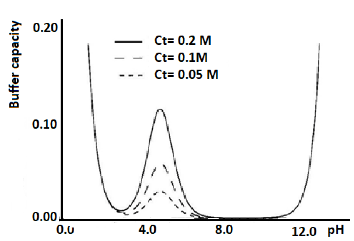
Figure 1: Variation of the buffer capacity vs. pH.
At intermediate values of the pH scale (between 4 and 10) and if Cs> 0.1, the values of [H+] and [OH-] can be neglected and:
Eq 4
The regulatory capacity reaches its maximum value when pH = log Ka, a relation that is deduced by setting the first derivative of the previous expression equal to zero; for this value, it is βmax = 2.303 Cs/4 = 0.576 Cs.
It follows from these relationships that the regulatory efficacy of a buffer:
a) It is directly proportional to the total concentration of the buffer system Cs; the higher said concentration, the greater the regulatory capacity.
b) Depends on the Cb/Ca concentration ratio; the closer this ratio is to the unit, the closer the pH value will be to that of log Ka and the greater the buffer capacity. In practice, this ratio is kept between 0.1 and 10, with which it is possible to modify the pH of the buffered systems by about two units simply by varying the ratio of acid to salt.
In Figure 1 it is observed that the most concentrated solution is the one with the greatest regulatory capacity and that this is the maximum for pH = log Ka.
To prepare a buffer solution of a given pH, an acid is chosen whose log Ka is as close as possible to the desired pH value. Equivalent amounts of this acid and its alkali salts are dissolved for maximum regulatory efficiency. The pH of the solution is obtained in the first approximation from the Henderson equation since the effect of ionic strength must be taken into account. Therefore, the resulting final value is not calculated but is determined experimentally. Perrin [9] has published a very useful book on buffers for use in various applications.
- Quite often, especially in the case of applying electrochemical methods, it is convenient to prepare buffers of known ionic strength, for which an inert salt of suitable concentration is added [10]. Studies have also been published in which the adjustment of the ionic strength has been carried out by calculating the appropriate amounts of Ca and Cb from the conjugated acid-base pair [7]. In supplement file 3 the program has been adapted to run under Windows 10. The backgrounds and equations used in this program have been explained in reference [4]. When running this program it makes the following question (values introduced for the acetate/HCl buffer have been included as an example): Buffer name (acetate will be saved in the output file name)
- Output file name (acetate.res where to save all introduced data and results of the calculations)
- Ionic strength (0.1 M, the selected one to be adjusted without the need for any inert salt)
- Proton number (1, number of protons participating in the system)
- More basic form charge (-1)
- More basic form size (3.5 as unknown)
- Log K (4.76)
- Acid form size (3.5 as unknown)
- Type of system buffer (strong acid/A)
- Basic form charge (-1)
- Acid form charge (0)
- Acid concentration (0.2 mol L-1)
- Base concentration (0.2 mol L-1)
- Total volume (to prepare 100 mL)
- Low pH (initial pH to calculate 3.2)
- Upper pH (last pH to calculate 6.0)
- pH step (0.2)
- Using this data, Table 1 is showing the obtained file.
| Table 1: Acetate buffer of a 0.1 M ionic strength using sodium acetate 0.2 mol L-1 and HCl 0.2 mol L-1 Buffer acetic Ionic strength 0.10 M. | |||
| Log K1= 4.760 | |||
| Acid concentration= 0.2 M Base concentration= 0.2 M Total volume= 100 mL | |||
| pH | V1 | V2 | β |
| 3.200 | 48.305 | 49.627 | 0.009260 |
| 3.400 | 47.359 | 49.765 | 0.012603 |
| 3.600 | 45.933 | 49.852 | 0.017887 |
| 3.800 | 43.841 | 49.907 | 0.025295 |
| 4.000 | 40.890 | 49.941 | 0.034575 |
| 4.200 | 36.948 | 49.963 | 0.044579 |
| 4.400 | 32.050 | 49.977 | 0.053082 |
| 4.600 | 26.486 | 49.986 | 0.057415 |
| 4.800 | 20.771 | 49.991 | 0.055946 |
| 5.000 | 15.478 | 49.995 | 0.049227 |
| 5.200 | 11.025 | 49.997 | 0.039583 |
| 5.400 | 7.573 | 49.998 | 0.029593 |
| 5.600 | 5.061 | 49.999 | 0.020947 |
| 5.800 | 3.317 | 50.000 | 0.014262 |
| 6.000 | 2.146 | 50.000 | 0.009456 |
Figure 2 represents the buffer capacity vs. the pH for the acetate buffer
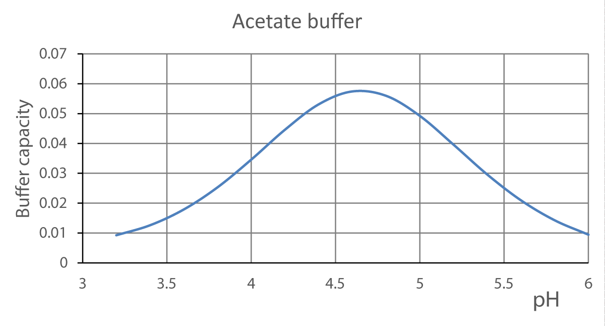
Figure 2: Buffer capacity vs. pH for the acetate buffer. HCl 0.2 mol L-1, NaOH 0.2 mol L-1 total volume= 100 mL.
Figure 3 and Table 2 show the results obtained for the citrate buffer used as an example of the application of the program to a polyprotic acid. In order to evidence the accuracy, the calculated pH values of the citrate buffer are compared with the obtained experimental values.
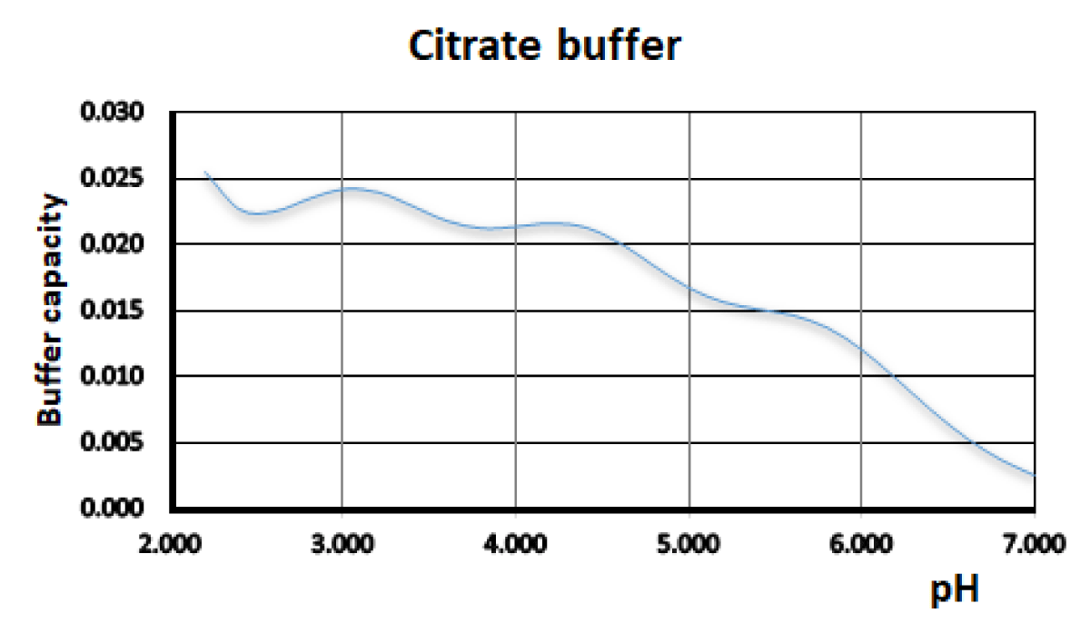
Figure 3: Buffer capacity vs. pH for the sodium citrate buffer. HCl 0.2 mol L-1, NaOH 0.2 mol L-1, total volume= 100 mL. Ionic strength 0.1 M.
| Table 2: Sodium citrate buffer capacity vs. pH. HCl 0.2 mol L-1, sodium citrate 0.07 mol L-1, Total volume= 100 mL. Ionic strength 0.1 M. | |||||||
| Citrate Buffer | HCl | Citrate | |||||
| pHtheor | pHexper | pHtheor - pHexper | VHCl | Vcitrate | VHCl + Vcitrate | VH2O to add to get 100 mL | Beta |
| 2.200 | 2.236 | -0.036 | 47.922 | 44.050 | 91.972 | 8.028 | 0.025506 |
| 2.400 | 2.426 | -0.026 | 46.628 | 45.350 | 91.978 | 8.022 | 0.022676 |
| 2.600 | 2.629 | -0.029 | 45.354 | 46.147 | 91.501 | 8.499 | 0.022527 |
| 2.800 | 2.833 | -0.033 | 43.491 | 46.605 | 90.096 | 9.904 | 0.023494 |
| 3.000 | 3.020 | -0.020 | 41.300 | 46.809 | 88.109 | 11.891 | 0.024228 |
| 3.200 | 3.215 | -0.015 | 38.902 | 46.790 | 85.692 | 14.308 | 0.023992 |
| 3.400 | 3.411 | -0.011 | 31.243 | 46.540 | 77.783 | 22.217 | 0.022936 |
| 3.800 | 3.807 | -0.007 | 31.243 | 45.225 | 76.468 | 23.532 | 0.021261 |
| 4.000 | 4.010 | -0.010 | 28.466 | 44.108 | 72.574 | 27.426 | 0.021386 |
| 4.200 | 4.205 | -0.005 | 25.524 | 42.710 | 68.234 | 31.766 | 0.021642 |
| 4.400 | 4.399 | 0.001 | 22.500 | 41.113 | 63.613 | 36.387 | 0.02132 |
| 4.600 | 4.595 | 0.005 | 19.551 | 39.433 | 58.984 | 41.016 | 0.020113 |
| 4.800 | 4.788 | 0.012 | 16.812 | 37.763 | 54.575 | 45.425 | 0.018356 |
| 5.000 | 4.982 | 0.018 | 14.353 | 36.136 | 50.489 | 49.511 | 0.016709 |
| 5.200 | 5.179 | 0.021 | 12.121 | 34.527 | 46.648 | 53.352 | 0.015637 |
| 5.400 | 5.367 | 0.033 | 10.047 | 32.898 | 42.945 | 57.055 | 0.015103 |
| 5.600 | 5.572 | 0.028 | 8.087 | 31.250 | 39.337 | 60.663 | 0.01464 |
| 5.800 | 5.778 | 0.022 | 6.267 | 29.643 | 35.910 | 64.090 | 0.01369 |
| 6.000 | 5.984 | 0.016 | 4.655 | 28.177 | 32.832 | 67.168 | 0.012008 |
| 6.200 | 6.188 | 0.012 | 3.320 | 26.941 | 30.261 | 69.739 | 0.009783 |
| 6.400 | 6.404 | -0.004 | 2.286 | 25.974 | 28.260 | 71.740 | 0.007441 |
| 6.600 | 6.598 | 0.002 | 1.532 | 25.263 | 26.795 | 73.205 | 0.00535 |
| 6.800 | 6.788 | 0.012 | 1.007 | 24.766 | 25.773 | 74.227 | 0.003687 |
| 7.000 | 6.990 | 0.010 | 0.052 | 24.300 | 24.352 | 75.648 | 0.002466 |
Universal buffers
The van Slyke equation shows that the buffering capacity is the sum of the contribution of the systems H2O/OH-, H3O+/H2O y HA/A-. Similarly, it can be shown that a property of buffers is that the total buffer capacity is the sum of the contribution of each of the acid-base systems. Thus for a mixture of monoprotic systems, one has [4]:Eq 5
Since each acid-base system buffers a zone of about 2.5 pH units centered on the log Ka value, if one wants to have a buffer system throughout the pH zone, he should select several conjugated acid-base pairs so that each of them covers an appropriate pH zone. In the case of the Prideaux buffer [11,12] (also erroneously cited as Britton-Robinson buffer), acetic acid (log Ka = 4.76), phosphoric (log K1 = 2.15; log K2 = 7.20; log K3 = 12.35) and boric acid (log Ka= 9.23) are mixed.
Figures 4-6 shows the variation in the regulatory capacity of the Prideaux buffer as a function of pH, observing that it practically does not disappear in any pH zone.
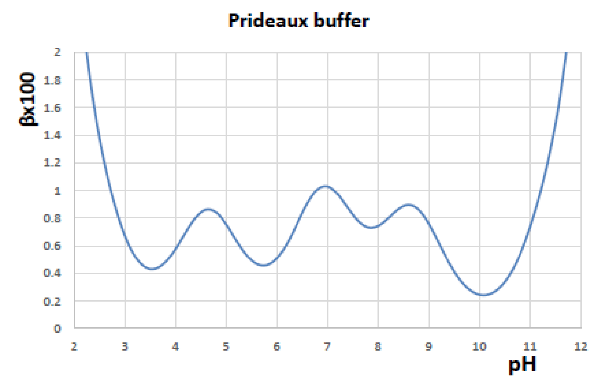
Figure 4: Buffer capacity of the Prideaux buffer.
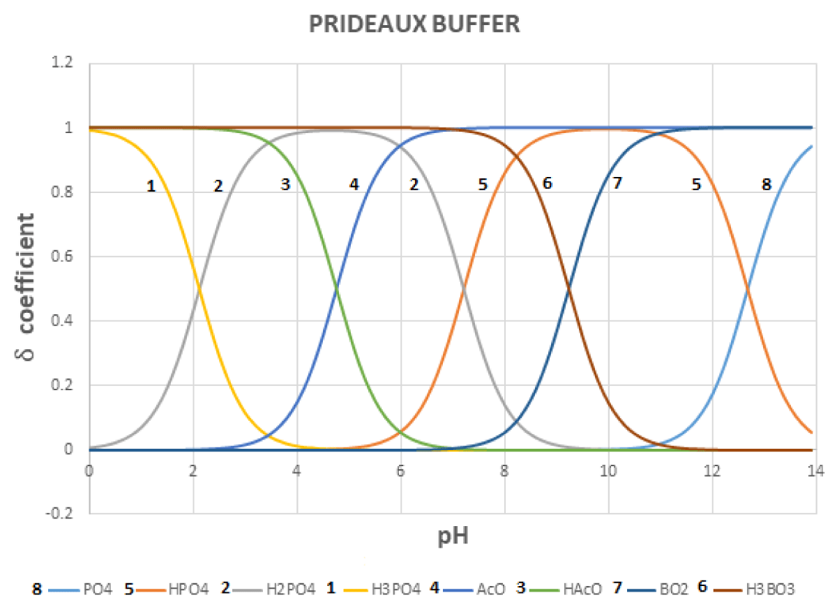
Figure 5: Distribution diagram for the Prideaux buffer.
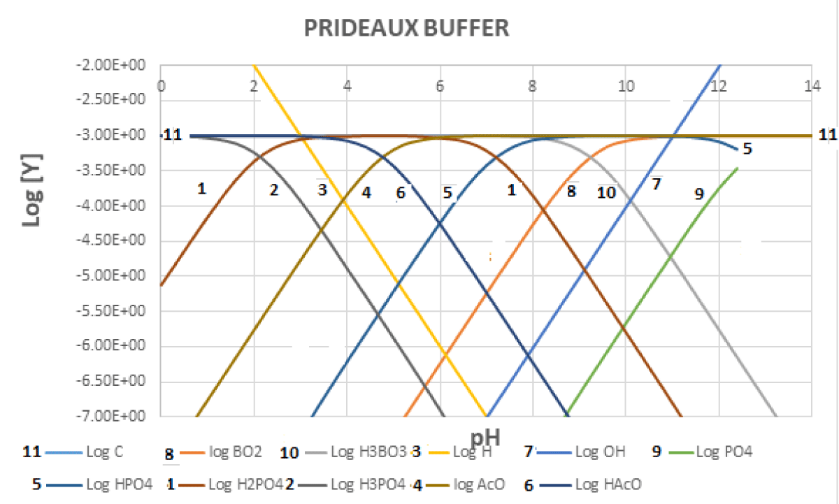
Figure 6: Logarithmic concentrations for the Prideaux buffer. The analytical concentration for each component is 0.001 mol L-1.
Brömsted method
Monoprotic acids: The pH of an acidic or basic solution can be calculated by proposing a general equation that relates it to the self-protolysis constant of the solvent, the concentration of the acid-base system, and its protonation constant [13,14].
For a mixture consisting of an acid HA with a Ca concentration and the sodium salt of its conjugated base NaA with a Cb concentration, there are four unknown concentrations in the medium: [HA], [A-], [H+], and [OH-]. The acidity protonation constant of the acid-base equilibrium will be given by
(h is used instead of [H+])
Note: It has not to be confused [HA] with Ca, or [A-] with Cb: the terms in brackets refer to the concentrations of the species at equilibrium, while the others are those that can be calculated from the quantities weighed at prepare the solutions or learn about them by analysis (hence they are called analytical concentrations). The total analytical concentration of the acid-base system will be Cs = Ca + Cb.
To calculate any of the unknown concentrations, for example, h, the solution charge balance may be established:
[Na+] + h = Cb + h = [OH-] + [A-]
If the distribution coefficient of [A-] is defined as:
Resulting:
Substituting in the charge balance:
Which is the expression of the Brönsted equation for a monoprotic system. To calculate the pH a third-degree equation must be solved:
Ka h3 + (1+Ka Cb) h2 - (Ca+Ka Kw) h - Kw = 0 Eq 6
Which may be done by applying the iterative Newton-Raphson method. However, some simplifications can be made taking into account the particular working conditions.
Brömsted program
In this paper, a Brömsted program has been developed to run under Windows 10 environment [15] (Included in supplement file 1). This program makes the following questions:
1. Name of the output file name where one wants to save the results
2. If one wants to follow the iterative process
3. The ionic product of water or solvent (pKW, or pKS)
4. The acidity dissociation constant of the acid, pKa
5. The acid concentration of the conjugated system
6. The base concentration of the conjugated system
After providing this data, the program generates the pH values and requests if one wants to calculate the pH for another set of concentrations. As a title example see Table 3 for a calculation made for the acetic/acetate system
| Protonation constants at 15 ºC | I = 0 | I = 0.1 M | |
| Water | pKw | 13.997 | 13.815 |
| Citric acid | Log K1 | 6.396 | 5.841 |
| Log K2 | 4.761 | 4.415 | |
| Log K3 | 3.128 | 2.941 |
| Table 3: pH values calculated with the BRÖMSTED program for the acetic/acetate system |
| pH calculation of the acid-base system: acetic/acetate pKw= 14.000 pKa= 4.750 |
| Acid concentration= 1.00 Base concentration= 0.00 pH= 2.376 |
| Acid concentration= 0.80 Base concentration= 0.20 pH= 4.148 |
| Acid concentration= 0.60 Base concentration= 0.40 pH= 4.574 |
| Acid concentration= 0.50 Base concentration= 0.50 pH= 4.750 |
| Acid concentration= 0.40 Base concentration= 0.60 pH= 4.926 |
| Acid concentration= 0.20 Base concentration= 0.80 pH= 5.352 |
| Acid concentration= 0.00 Base concentration= 1.00 pH= 9.375 |
Diprotic acids: For a diprotic acid, we have
Eq 7
If we call
And take into account the charge balance as:
h + C1 + 2C2= [HA-]+ 2[A2-]+[OH-]
and the distribution coefficients as:
Then, substituting in (1)
And finally
β22h4+(β1+C1β2+2C2β2)h3+(1+C1β1+2C2β1-β2KW-Csβ1)h2+(C1+2C2- β1KW-2Cs)h - KW = 0 Eq 8
Which may be solved again by applying the iterative Newton-Raphson method Table 4.
| Table 4: Bronsted pH calculation for diprotic systems. |
| pH calculation for succinic acid/sodium succinate pKw= 14.000 pK1= 4.210 pK2= 5.640 |
| H2A conc.= 0.050 NaHA conc.= 0.000 Na2A conc.= 0.000 pH= 2.763 |
| H2A conc.= 0.050 NaHA conc.= 0.010 Na2A conc.= 0.000 pH= 3.519 |
| H2A conc.= 0.050 NaHA conc.= 0.050 Na2A conc.= 0.000 pH= 4.169 |
| H2A conc.= 0.050 NaHA conc.= 0.050 Na2A conc.= 0.010 pH= 4.373 |
| H2A conc.= 0.050 NaHA conc.= 0.050 Na2A conc.= 0.050 pH= 4.925 |
| H2A conc.= 0.050 NaHA conc.= 0.000 Na2A conc.= 0.050 pH= 4.925 |
| H2A conc.= 0.050 NaHA conc.= 0.010 Na2A conc.= 0.050 pH= 4.925 |
| H2A conc.= 0.000 NaHA conc.= 0.050 Na2A conc.= 0.000 pH= 4.925 |
| H2A conc.= 0.010 NaHA conc.= 0.050 Na2A conc.= 0.050 pH= 5.477 |
| H2A conc.= 0.000 NaHA conc.= 0.050 Na2A conc.= 0.050 pH= 5.682 |
| H2A conc.= 0.000 NaHA conc.= 0.000 Na2A conc.= 0.050 pH= 9.169 |
A new program to calculate the composition of buffer solutions of known ionic strength without the need of adding an inert salt has been developed. A list of different buffers has been included in supplementary material 2. In any case, the calculated buffer values have always to be validated making the corresponding experimental experiments. Usually, very small differences are found between the calculated and experimental values.
The pH of conjugated acid-base solutions may be calculated using the Newton-Raphson iterative method applied to the Brönsted equations. To calculate the composition of buffer systems two different methods may be applied, one using the Henderson-Hasselbach equation, and the other using the Brönsted equation. Usually, the simple Henderson-Hasselbach equation may be applied for the intermediate pH zone of the pH scale, but the third-degree Brönsted equation has to be used in the overall pH scales, especially on both sides of the pH scale.
- De Ford D, Anderson DL. The Effect of Ionic Strength on Polarographic Half-wave Potentials. J Amer Chem Soc. 1950; 72: 3918.
- Elving PJ, Komyathy JC, Van Atta RE, Ching-Siang Tang I. Rosenthal. Polarographic Behavior of Organic Compounds. Anal Chem. 1951; 23: 1218.
- Kemula W, Axt-Zak A. Roczniki Chem. 1964; 38: 683.
- Nath A, Bhattacharya AK. Indian J Chem. 1964; 2: 419.
- McIlvane TC. A buffer solution for colorimetric comparison. J Biol Chem. 1921; 49: 183-186.
- Meites L. Handbook of Analytical Chemistry. McGraw-Hill. New York, 1963. 1st edition.
- Britton HTK. Robinson RA. J Chem Soc. 1931; 1456.
- Mongay C, Cerdà V. A generalized calculation for preparation of buffer solutions of known ionic strength. Computers & Chemistry. 1984; 8: 213‑216
- Perrin DD. Buffers for pH and Metal Ion Control. Chapman and Hall. 1974. ISBN 0 412 11700 2
- Phansi P, Mongay C, Cerdà V. Buffers of formate, acetate and citrate of know ionic strength. Current Topics in Electrochemistry. 2019; 21: 107-117
- Mongay C, Cerdà V. VI/A Britton‑Robinson Buffer of Known ionic strength. Ann Chimica. 1974; 64: 409.
- Cerdà V, Mongay C. Preparation of a universal buffer of ionic strength 0'3 M. Talanta. 1977; 24: 747 748.
- Freiser H, Fernando Q. Ionic equilibria in Analytical Chemistry. John Wiley, New York, 1963.
- Mongay C, Cerdà V. I Introduction to Analytical Chemistry. Teaching materials collection 106. University of the Balearic Islands. 2004. ISBN 84-7632.862-1
- Brönsted program. www.sciware-sl.com