
More Information
Submitted: November 21, 2025 | Approved: December 08, 2025 | Published: December 09, 2025
How to cite this article: Segoloni E. An Original FORTRAN Code Combined with an XMGRACE© Graphical Routine Aimed at the Parameter Calculations and Drawing of Newton Diagrams for Crossed Molecular Beams (CMB) Experiments Planning. Ann Adv Chem. 2025; 9(1): 042-048. Available from:
https://dx.doi.org/10.29328/journal.aac.1001059
DOI: 10.29328/journal.aac.1001059
Copyright license: © 2025 Segoloni E. This is an open access article distributed under the Creative Commons Attribution License, which permits unrestriCted use, distribution, and reproduCtion in any medium, provided the original work is properly cited.
Keywords: Crossed Molecular Beams (CMB); Newton diagrams; Reaction dynamics; Center-of-mass transformations; Kinematic analysis of chemical reactions; FORTRAN computational code; Scattering angle calculations; Classical collision theory; Molecular beam kinematics; Graphical visualization of reaction dynamics

An Original FORTRAN Code Combined with an XMGRACE© Graphical Routine Aimed at the Parameter Calculations and Drawing of Newton Diagrams for Crossed Molecular Beams (CMB) Experiments Planning
Enrico Segoloni*
Former PhD Student and Post-DOC Researcher at Perugia University, Department of Chemistry, Italy
*Address for Correspondence: Enrico Segoloni, Former PhD Student and Post-DOC Researcher at Perugia University, Department of Chemistry, Italy, Email: [email protected]
This work presents a detailed computational method for analyzing and visually representing molecular collision dynamics in crossed molecular beam (CMB) experiments. An original UNIX-based FORTRAN code was created to calculate important kinematic parameters and build Newton diagrams for reactive systems where two monoenergetic beams intersect at any angle between 0° and 180°. The program finds center-of-mass velocities, collisional energies, product scattering velocities, angular ranges, and coordinate changes between laboratory and center-of-mass reference frames, using the principles of classical mechanics. A related XMGRACE-compatible routine creates high-resolution Newton diagrams that are ready for publication. This allows users to visualize reaction kinematics, scattering circles, and time-of-flight (TOF) detection angles accurately. An extra DOS/GW-Basic executable is included for quick on-screen visualization. The method has been thoroughly tested with different reactive channels and various chemical systems. By combining analytical derivations with automated graphical output, the tool provides a flexible platform for planning CMB experiments, interpreting dynamic results, and comparing theoretical predictions with observed scattering behavior. The codes are free for scientific use with proper credit.
Newton Diagrams are vector representations of the collisional events between two particles treated based on classical physics. Such types of diagrams are extensively used for the planning and the cinematic analysis of collisional events that typically occur in Crossed Molecular Beams (CMB) experiments performed in a high vacuum environment, which are at the basis of the Reaction Dynamics investigations [1-7].
The present work describes in detail a UNIX-based code aimed at the collisional parameter calculation and at the drawing of Newton Diagrams for two reacting molecular beams intersected at any angle g between 0 and 180 degrees. The global code, written in FORTRAN, was implemented by the author during his Ph.D. course in Chemistry and has been used and tested for a great variety of reactions.
It consists of two main parts: The first one calculates the reaction parameters of two monoenergetic beams of particle interacting at a given angle g, for a given elementary reaction; the second one generates and save an XMGRACE©-readable file which after the launch/opening of an UNIX© executable, draws an high-resolution graphical scheme of the reactions knematics, which in turn can be modified, printed or exported in the desired format for its final inclusion in a publication.
Moreover, it is also alleged to be a simple GW-Basic©/DOS© executable which can generate a Newton Diagram for a quick on-screen visualization for a given reaction.
The codes cited in this article can be freely used or copied by the reader(s), provided that due credit is given by the user(s) to the author.
II. Theoretical treatment of the collision of two particles, according to the classical physics
II.a. Vector derivation of the expressions for Center-Mass velocity (Vc.m.) and angle (Qc.m.): Considering the generic reaction:
A + BC → AB + C (I)
Between two particle reagent beams A and BC crossed at whatever angle g (with 00 g< 1800) e with velocities VA e VBC, for the conservation of the linear momentum in the C.M. reference system:
mAUA + mBC<gBC = 0 (A.I.1)
And the vectorial differences:
UA = VA - Vc.m. (A.I.2a)
UBC = VBC - Vc.m. (A.I.2b)
(Figure II.1.) We obtain from (A.I.1):
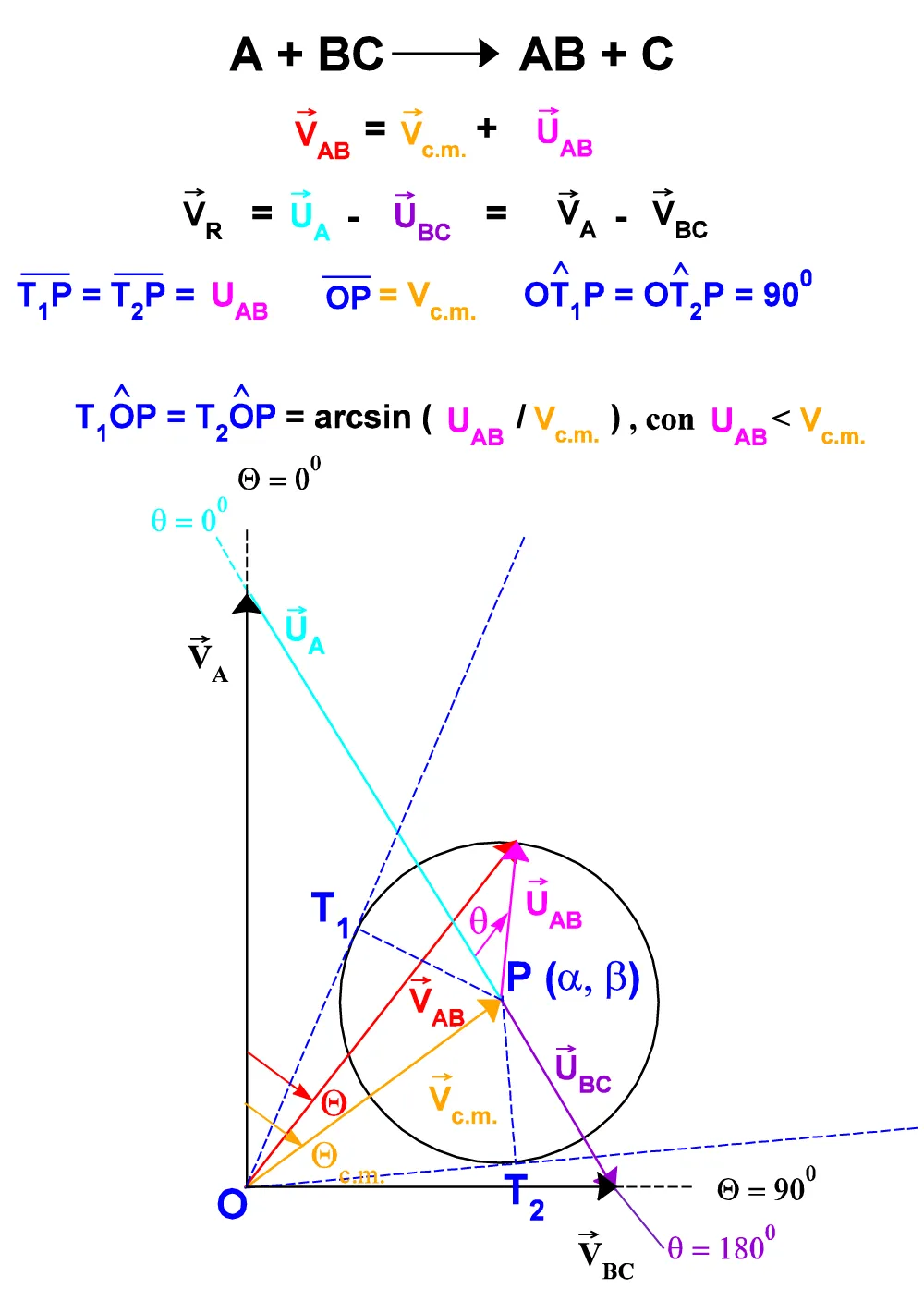
Figure A.II.1: Vectorial relations for the generic reaction: A + BC → AB + C.
mAVA - mAVc.m. + mBCVBC - mBCVc.m. = 0
Namely:
Vc.m. = (mAVA + mBCVBC) / (mA + mBC) (A.I.3)
Using the unit vectors i, j for representing VA and VBC (Figure A.I.1), for g = 900:
VBC = VBC i (A.I.4a)
VA = VA j (A.I.4b)
By substituting the (A.I.4a, b) into (A.I.3):
Vc.m. = [(mBCVBC)/(mA+mBC)]( i ) + [(mAVA)/(mA+mBC)]( j ) (A.I.5)
By expressing the vector Vc.m. as a function of its components parallel to the X and Y axes of the Laboratory reference system:
Vc.m. = [a]( i ) + [b]( j ) (A.I.6)
The modules of these component vectors a e b correspond to the Cartesian coordinates of the point P (the tip of the Vc.m. vector) in the reference system XOY.
By confronting (A.I.5) with (A.I.6) we get:
a = (mBCVBC) / (mA+mBC) e b = (mAVA) / (mA+mBC) (A.I.7)
Moreover, by letting pBC = mBCVBC and pA = mAVA,:
Vc.m. = (pA2 + pBC2)1/2 / (mA + mBC) (A.I.8a)
and
tan (Qc.m.) = (a / b) = (pBC / pA) (A.I.8b)
For 00 < g <900, we have:
VBC = (VBC)Xi + (VBC)Yj (A.I.9a)
VA = VA j (A.I.9b)
The modules of the component vectors of VBC are given by:
(VBC)X = vBCsin g; (VBC)Y = VBCcos g (A.I.10a,b)
By substituting the (A.I.10a, b) into (A.I.9a) and then the (A.I.9a, b) into (A.I.3), we obtain:
Vc.m. = [(mBCVBCsing)(i)+(mAvA+mBCVBCcosg)(j)]/(mA+mBC), (A.I.11)
from which:
a = (mBCVBCsin g) / (mA+mBC), (A.I.12a)
b = (mAVA+mBCVBCcos g) / (mA+mBC) (A.I.12b)
And:
Vc.m.=(pA2+pBC2+2pApBCcosg)1/2/(mA+mBC) (A.I.13)
For 900 < g <1800:
VBC = (VBC)X i + (VBC)Y (-j) (A.I.14a)
VA = VAj (A.I.14b)
The modules of the component vectors of vBC are given by:
(VBC)X = VBCsin g (A.I.15a)
(VBC)Y = - VBCcos g (A.I.15b)
By substituting the (A.I.15 a,b) into (A.I.14a) and then the (A.I.14a,b) into (A.I.3), we get the (A.I.11) again:
Vc.m.=[(mBC·VBCsing)(i)+(mA·vA+mBC·VBC·cosg)(j)]/(mA+mBC), (A.I.11)
the (A.I.12a,b):
a = (mBC·VBCsing) / (mA+mBC),
b = (mA·VA+mBC·VBCcos g) / (mA+mBC)
And the:
Vc.m.= (pA2 + pBC2 + 2pA·pBCcos g)1/2 /(mA+mBC) (A.I.13)
Generally, it is more convenient to express the Qc.m. angle as a function of VA, Vc.m., and uA rather than directly as the arctangent of the ratio a / b, because in this fashion it can be obtained a single general formula effective for each value of g between 00 and 1800.
Based on a generic reactive system geometry (Figure I.2.; Figure II.2.), we have:
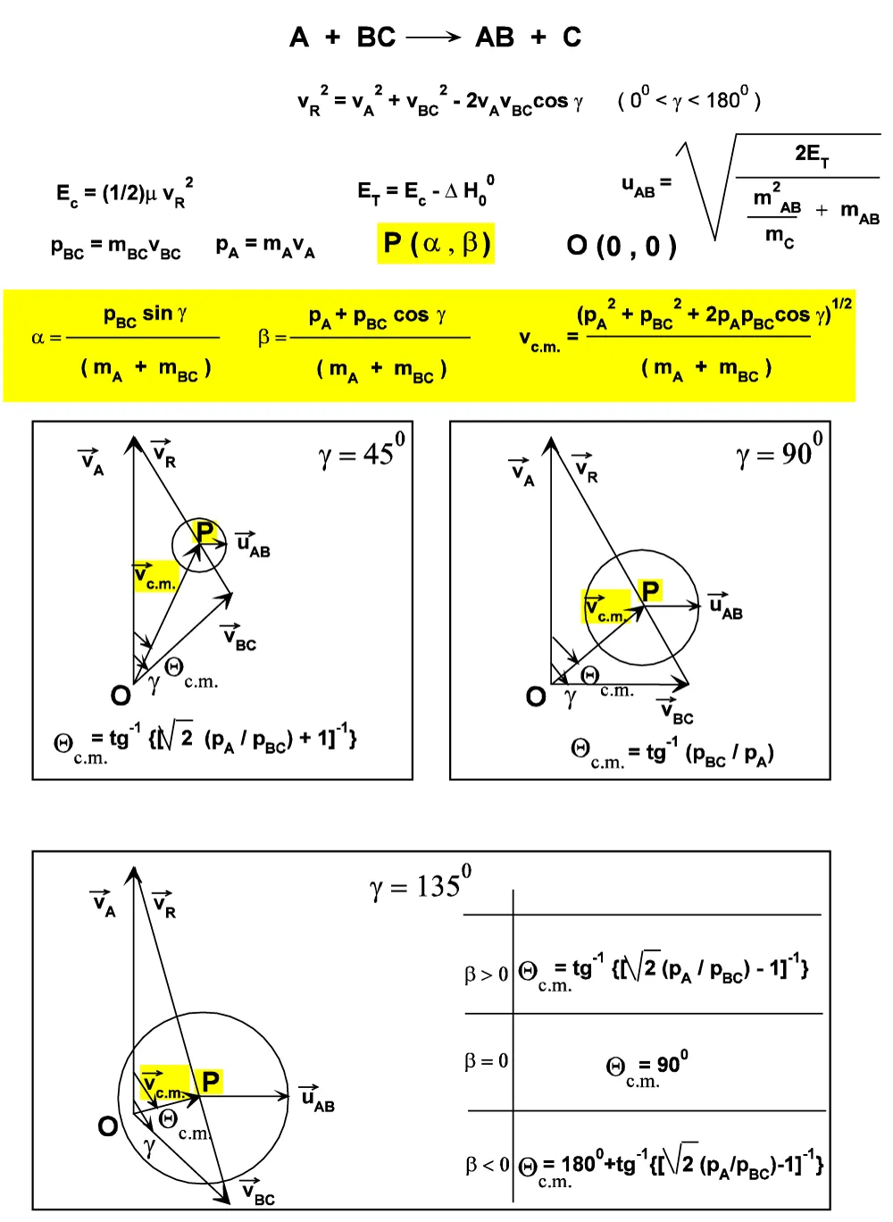
Figure. A.II.2: Θc.m. values for γ = 45°, 90° and 135°.
UA2 = VA2 + Vc.m.2 - 2 VA · Vc.m.cos(Qc.m.) (A.I.14)
hence:
Qc.m.= arccos[(VA2 + Vc.m.2 - UA2) / (2 VA· Vc.m.)]. (A.I.15)
But:
Vc.m.2 = a2 + b2 and UA2 = a2 + (VA - b)2
Then:
Qc.m.= arccos[(b) / (a2 + b2)]. (A.I.16)
By substituting into (A.I.16) the (A.I.12a, b) we obtain finally:
Qc.m.= arccos[(pA + pBCcos g) /(pA2 + pBC2 +
+ 2pA·pBC·cos g)1/2], (A.I.17)
Valid for each g between 00 and 1800.
II.b. Relations between the Cartesian coordinate system of the Center of Mass and the Laboratory system for a generic point P in the velocity plane.
The Center of Mass reference system can be seen as the result of a translation of the origin O(0,0) of the Laboratory reference system axes VxLAB, VyLAB into the point P(a, b), which is the Center of Mass followed by an anti-clockwise rotation of f degrees (Figure A.II.1), where f is given by :
f = arctan(VBC sing / [VA - VBC cosg]) (A.II.1)
and 00 < g < 1800.
It follows that the relations which allow the passage from Center of Mass coordinates to the Laboratory ones for a generic point P are given by:
VxLAB = Vxc.m. cos f - Vyc.m. sin f + a (A.II.2 a,b)
VyLAB = Vxc.m. sin f + Vyc.m. cos f + b
II.b.1. Relations between Cartesian and Polar Coordinates in the two reference systems
Based on Figure A.II.1, we can also write:
VxLAB = VP sin Q (A.II.3)
VyLAB = VP cos Q
And:
Vxc.m. = UP sin q (A.II.4)
Vyc.m. = UP cos q
Where VP, UP are respectively the P product velocity in the Laboratory reference system and in the Center of Mass one and Q e q the corresponding angles.
By substituting the (A.II.3) and (A.II.4) into (A.II.2), we have:
VP sin Q = UP sin q cos f - UP cos q sin f + a (A.II.5)
VP cos Q = UP sin q sin f + UP cos q cos f + b
Namely:
VP sin Q = UP sin( q - f ) + a (A.II.6 a, b)
VP cos Q = UP cos(q - f ) + b
Dividing member by member the (A.II.6):
tan Q = (UP sin( q - f ) + a) / (UP cos( q - f ) + b) (A.II.7)
By combining the (A.II.6 a, b) as a function of the angle Q:
tan (q - f) = (VP sin(Q) - a) / (VP cos(Q) - b) (A.II.8)
A.II.3. Jacobian operator and relations for the conversion of the Laboratory reference frame angles Q into the Center of Mass reference system ones.
Between the product flux in the two reference systems, the following relation holds:
ILAB(Q,VP) = (VP2/UP2)· Ic.m.(q,UP) (A.II.9)
The product's density measured in the Laboratory reference system is:
N(Q,VP) = (VP/UP2)· Ic.m.(q,UP) (A.II.10)
Where (V2/U2) is the Jacobian operator, which converts the effective Center of Mass flux into the one observed in the Laboratory reference frame.
By expressing the velocity of a generic product’s particle P as VP in the Laboratory frame as a function of the corresponding velocity in the Center of Mass reference system UP and of the Center of Mass velocity Vc.m. :
VP2 = UP2 + Vc.m.2 - 2UP ·Vc.m. cos w. (A.II.11)
Where w is the {OPK} triangle angle defined by the half-lines where are the vectors UP and Vc.m. (Figure A.II.3.). The expressions for w as a function of the angle Q formed by the vectors VP and VA are given by:
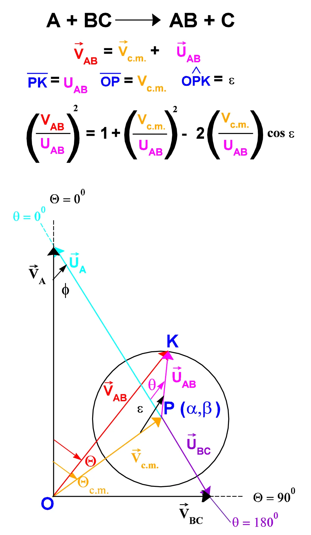
Figure. A.II.3: “Jacobian” operator.
w = p - f - Qc.m. + q for Q < Qc.m.
w = p for Q = Qc.m.
w = p + f + Qc.m. - q for Q > Qc.m. (A.II.12 a, b, c)
Dividing each part of (A.II.11) by UP2, it can be obtained the expression for the "Jacobian" as a function of w:
(VP2/UP2) = 1 + (Vc.m. / UP)2 - 2(Vc.m. / UP) cos w. (A.II.13)
or:
(VP/UP2) = {[1 + (Vc.m. / UP)2 - 2(Vc.m. / UP) cos w]½}/UP (A.II.14)
Applying the sine’s theorem to the same triangle {OPK} above, by varying the angle, Q it is possible to obtain expressions for the conversion of the Q angles of the Laboratory system to the angles q of the center of Mass reference system (Figure A.II.4):
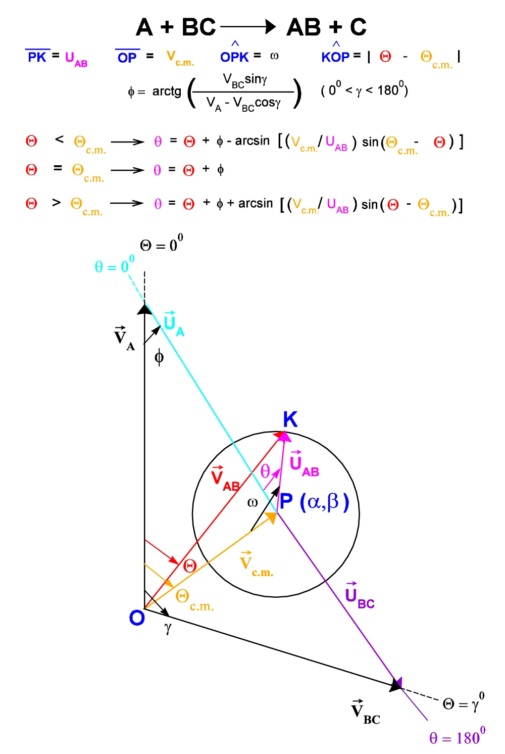
Figure. A.II.4: Laboratory and C.M. system vector relationships.
for Q < Qc.m. q = Q + f - arcsin {(Vc.m. / UAB)sin(Qc.m. - Q)}
for Q = Qc.m. q = Qc.m. + f
for Q > Qc.m. q = Q + f + arcsin {(Vc.m. / UAB)sin(Q - Qc.m.)}. (A.II.14 a, b, c)
A.II.4. Collisional energy (Ec), angular range amplitude (DA), velocity (vCM), and angle (QCM) of the center of mass dependence on g (intersection angle of the reagents beams).
Considering two reagent beams A and BC crossed at an angle g between 00 and 1800, the collisional energy is given by:
Ec = (½) m Vr2 (A.II.15)
Where m is the reduced mass of the reagents and their relative velocity:
Vr = (VA 2+VBC2- 2VA·VBC cos g)1/2 (A.II.16)
Ec as a function of g in the range (0, p) is in general always growing when the angle g increases, with a flection at the point (p/2, ½ m(VA2 + VBC2) of the plane {Ec, g}, corresponding to a beam configuration of 900. The velocity vector of a generic product AB in the Center of mass reference system is given by:
UAB = (2ET / [{mAB2 / mC} + mAB])1/2 (A.II.17)
Where the total energy ET is given by the sum of the collisional energy and the exothermicity of the considered reaction:
ET = (½)m Vr2 - DH00 (A.II.18)
It is always growing in the interval (0,p) of the angle g (Figure A.II.3b ). If the quantity:
(2VA·VBC) / (VA 2+ VBC2 - 2DH0) (A.II.19)
Is less then 1, the UAB = f(g) a flex point at g = (2VA VBC) / (VA 2+VBC2 - 2DH00).
The Vc dependence g is given by:
Vc.m. =(pA2 + pBC2 + 2pA·pBCcos g)1/2 / (mA+mBC) (A.II.20)
It is always decreasing when the value of g increases, with an inflexion point at gF = arccos(-py / px), if py/px < 1, and gF = arccos(-px/py) if py/px> 1, with 900 < g F £ 1800.
The angular range amplitude of a scattering circle with respect to the Laboratory frame is:
DA(g) = Qmax - Qmin = 2 arcsin (UP / Vc.m..) (A.II.23)
Where:
QMax = Qc.m. + arcsin (UP /Vc.m..) (A.II.21)
QMinMin = Qc.m. - arcsin (UP / Vc.m..). (A.II.22)
And Qc.m. is the center of mass vector angle, UP is the scattering velocity of the product P(= AB, C) with respect to the center of mass frame, and Vc.m. is the center of mass vector module.
The function DA(g) = 2 arcsin (UP / Vc.m..) (with UP £ Vc.m..) is always growing in the interval (0, gI), in cui gI is the limit angle (lesser than 1800) between the beams when uP = vc.m.. (isotachic point: iso - tachis =same velocity).
The general expression for the center of mass angle is given by:
Qc.m. = arccos[(pA + pBC·cos g) / (pA2 + pBC2 + 2pApBCcos g)1/2] (A.II.24)
By the substitution: R = (pA / pBC ), it can be written as:
Qc.m. = arccos[(R + cos g) / (R2 + 1 + 2Rcos g)1/2] (A.II.25)
It can be demonstrated that for reactions with 0
Qc.m. = g and Qc.m. = ½(g) (Figure A.II.5).
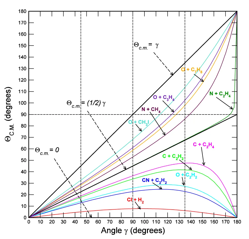
Figure. A.II.5: Θcm dependence from the crossing angle γ for some reactive systems.
Qc.m. = ½(g) is the (A.II.25) for R = 1, namely for those reactions with pA = pBC. If R > 1 (namely for ractions with pA > pBC), the corresponding curves Qc.m. = f(g) show a relative maximum for gMAX = arccos(-1 / R) = arccos(- pBC / pA), and are comprised between the two straight lines:
Qc.m. = ½(g), Qc.m. = 0.
For R tending to +¥, the curves Qc.m. = f(g) approximate to the line Qc.m. = 0, while for R tending to 0, they approach asymptotically the Qc.m. = g.
(Figure A.II.5)
III. Algorithm for the drawing of Newton Diagrams
Considering a generic reactive channel relative to a given multichannel reaction:
A + BC ® AB(i) + C(i)
Between two beams of reagents A and BC crossed at a whatever angle g (between 00 and 1800) with velocities VA and VBC, respectively. If N is the number of the global reaction, it is possible to define the following algorithm for the Newton Diagrams drawing:
Input data subroutine
Read:
masses velocities of the reagents: mA, VA, mBC, VBC
Angle between the two beams: g
number of reactive channels: N
TOF spectra angles number: NTOF
TOF spectra angles:
for i = 1 to NTOF { Q(i) } end
Produces masses and reactive channels’ Enthalpies:
For i = 1 to N { mABc00 (i) } end
Interval extremes for the drawing: VXmax=VYmax
SUBROUTINE for the cinematic parameters calculations
Calculate:
Reagents total mass: mT = mABC
Reagents reduced mass: m = mA · mBC / mT
Reagents linear momenta:
pBC = mBCVBC;
pA = mAVA
Scattering circles coordinates:
a = (pBC sin g) / mT ; b = ( pA + pBC cos g) / mT
Center of Mass velocity modulus:
Vc.m. = ( a2 + b2 )
Center of Mass velocity vector angle:
Qc.m.= arccos [(b) / (a2 + b2)].
Relative velocity modulus:Vr2 = VA 2+VBC2 -2VAVBCcos g
Collisional energy:
Ec = (1/2)mVr2
Total energies for the reactive channels: For i = 1 to N
{ET(i) = Ec - DH00 (i)}
end
Products scattering circles rays:
For = i = 1 a N
UAB (i) ={2ET/([ mAB 2 (i) / mC (i)] + mAB (i))}1/2 ;
UC (i) = ( mAB (i) / mC (i)) · UAB (i)
End
Reactive circles range EXTREMES angles SCATTERING calculation SUBROUTINE
Calculate:
For i = 1 to N
if UA B (i) £ Vc then
i-th Circle Angular range amplitude:
DA(i) = 2 · arcsin (UA B (i) / Vc.m. )
Minimum angle: Amin(i) = Qc.m. - DA(i) / 2
Maximum angle: Amax(i) = Qc.m. + DA(i) / 2
if UA B (i) > Vc.m. then i = i+1; continue
end
Coordinates of the scattering circles points calculations subroutine
Calculate:
For i = 1 to N
for q = 0 to 2p step (50 / 1800)·p
x(i) = a + UA B (i)· cos q
y(i) = b + UA B (i)· sin q
end
end
SUBROUTINE for the calculations of the limiting angles of the straight lines which define the RANGES of SCATTERING and of the TOF spectra angles
Calculate:
For i = 1 to N
for e = Amin(i), Amax(i), Q(i)
yR = Xmax·cos |e|
xR = yR / {tan([p/2]-e)}
end
SUBROUTINE for the T.O.F. spectra angles calculation in the Center of Mass reference system
Calcolate:
f = arctan (VBC sin g / [VA - VBC cos g])
for i = 1 to NTOF
if Q(i) < Qc.m. then
q(i) = Q(i) + f - arcsin {(Vc.m./UAB (j) )sin(Qc.m. - Q(i))}
if Q(i) = Qc.m. then
q(i) = Qc.m. + f
if Q(i) > Qc.m. then
q (i) = Q(i) + f + arcsin {(Vc.m./UAB (j))sin(Q(i) - Qc.m.)}
end
Evaluated results OUTPUT SUBROUTINE
Print:
Center of Mass angle of the C.M. velocity vector: Qc.m.
C. M. velocity vector modulus: Vc.m.
Collisional energy: Ec
Total energies of the N reactive channels ET(i)
Reagents' elastic scattering velocities:
VeA, VeBC
Products' maximum reactive scattering velocities:
UA B (i), UC (i)
Angular Ranges extremes of the scattering circles:
Amin(i), Amax(i)
(Figure A.III.1)
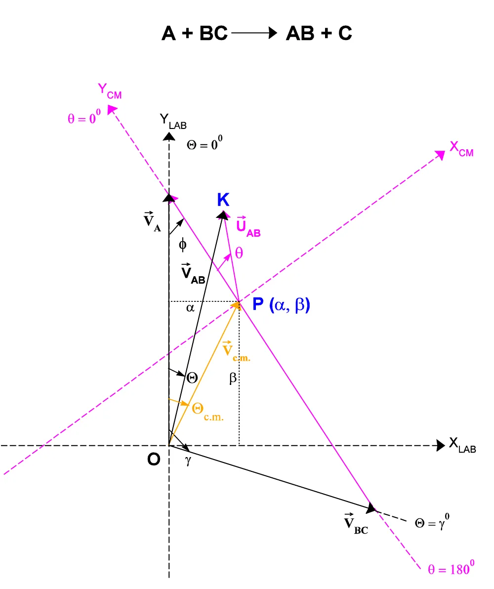
Figure. A.III.1: Relations between the Laboratory reference system coordinates and the Center of mass system ones.
Graphical Output:
Newton Diagram drawn in the velocity plane
between: (Vxmin, Vxmax) - (Vymin, Vymax)
(Figure A.III.2)
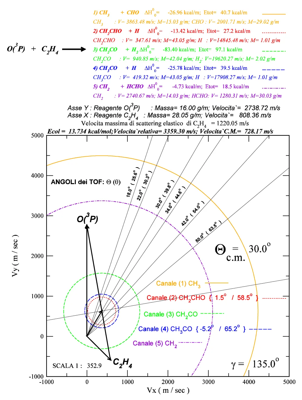
Figure. A.III.2: Example of graphical output obtained by the FORTRAN code and XMGRACE program.
- Fisk GA, McDonald JD, Herschbach DR. Discuss Faraday Soc. 1967;44:228.
- Polanyi JC. Some Concepts in Reaction Dynamics. Chemica Scripta. 1986;27:229. Available from: https://www.nobelprize.org/uploads/2018/06/polanyi-lecture.pdf
- Casavecchia P. Chemical reaction dynamics with molecular beams. Rep Prog Phys. 2000;63:355. Available from: https://iopscience.iop.org/article/10.1088/0034-4885/63/3/203/pdf
- Lee YT. Atomic and Molecular Beam Methods. In: Scoles G, editor. Vol. 1. New York: Oxford University Press; 1987;553–568.
- Parrish DD, Herschbach DR. J Am Chem Soc. 1973;95:6133.
- Sibener SJ, Buss RJ, Ng CY, Lee YT. Rev Sci Instrum. 1980;51:167.
- Levine RD, Bernstein RB. Molecular Reaction Dynamics and Chemical Reactivity. New York: Oxford University Press; 1987.